Supplemental Videos
The main topics of this section are also presented in the following videos:
The main topics of this section are also presented in the following videos:
It is often useful to consider trigonometric functions after we have applied function transformations to them. In this section we review function transformations and their effects on the equations and graphs of trigonometric functions.
If you would like to review function transformations in more depth, you can refer to Function Transformations5.
There are many situations (which we will see in later sections) where it is useful to consider functions such as \(j(x) = -2\sin(\pi(x-1))+3\text{.}\) We will work our way up to this function, but first let's start by exploring a simpler function, \(g(x) = 2\sin(x)\text{.}\) If we want to determine what the graph of \(g(x)\) looks like, we can start by finding a few points on the graph using a table.
\begin{equation*}
\theta
\end{equation*}
|
\begin{equation*}
\ \ \ 0 \ \ \
\end{equation*}
|
\begin{equation*}
\ \ \frac{\pi}{6} \ \
\end{equation*}
|
\begin{equation*}
\ \ \frac{\pi}{4} \ \
\end{equation*}
|
\begin{equation*}
\ \ \frac{\pi}{3} \ \
\end{equation*}
|
\begin{equation*}
\ \ \frac{\pi}{2} \ \
\end{equation*}
|
\begin{equation*}
\ \ \frac{2\pi}{3} \ \
\end{equation*}
|
\begin{equation*}
\ \ \frac{3\pi}{4} \ \
\end{equation*}
|
\begin{equation*}
\ \frac{5\pi}{6} \
\end{equation*}
|
\begin{equation*}
\ \ \ \pi \ \ \
\end{equation*}
|
\begin{equation*}
\ \frac{7\pi}{6} \
\end{equation*}
|
\begin{equation*}
\frac{5\pi}{4}
\end{equation*}
|
\begin{equation*}
\frac{4\pi}{3}
\end{equation*}
|
\begin{equation*}
\ \frac{3\pi}{2} \
\end{equation*}
|
\begin{equation*}
\sin(\theta)
\end{equation*}
|
\begin{equation*}
\ 0 \
\end{equation*}
|
\begin{equation*}
\frac{1}{2}
\end{equation*}
|
\begin{equation*}
\frac{\sqrt{2}}{2}
\end{equation*}
|
\begin{equation*}
\frac{\sqrt{3}}{2}
\end{equation*}
|
\begin{equation*}
1
\end{equation*}
|
\begin{equation*}
\frac{\sqrt{3}}{2}
\end{equation*}
|
\begin{equation*}
\frac{\sqrt{2}}{2}
\end{equation*}
|
\begin{equation*}
\frac{1}{2}
\end{equation*}
|
\begin{equation*}
\ 0 \
\end{equation*}
|
\begin{equation*}
-\frac{1}{2}
\end{equation*}
|
\begin{equation*}
-\frac{\sqrt{2}}{2}
\end{equation*}
|
\begin{equation*}
-\frac{\sqrt{3}}{2}
\end{equation*}
|
\begin{equation*}
-1
\end{equation*}
|
\begin{equation*}
2\sin(\theta)
\end{equation*}
|
\begin{equation*}
\ 0 \
\end{equation*}
|
\begin{equation*}
1
\end{equation*}
|
\begin{equation*}
\sqrt{2}
\end{equation*}
|
\begin{equation*}
\sqrt{3}
\end{equation*}
|
\begin{equation*}
2
\end{equation*}
|
\begin{equation*}
\sqrt{3}
\end{equation*}
|
\begin{equation*}
\sqrt{2}
\end{equation*}
|
\begin{equation*}
1
\end{equation*}
|
\begin{equation*}
\ 0 \
\end{equation*}
|
\begin{equation*}
-1
\end{equation*}
|
\begin{equation*}
-\sqrt{2}
\end{equation*}
|
\begin{equation*}
-\sqrt{3}
\end{equation*}
|
\begin{equation*}
-2
\end{equation*}
|
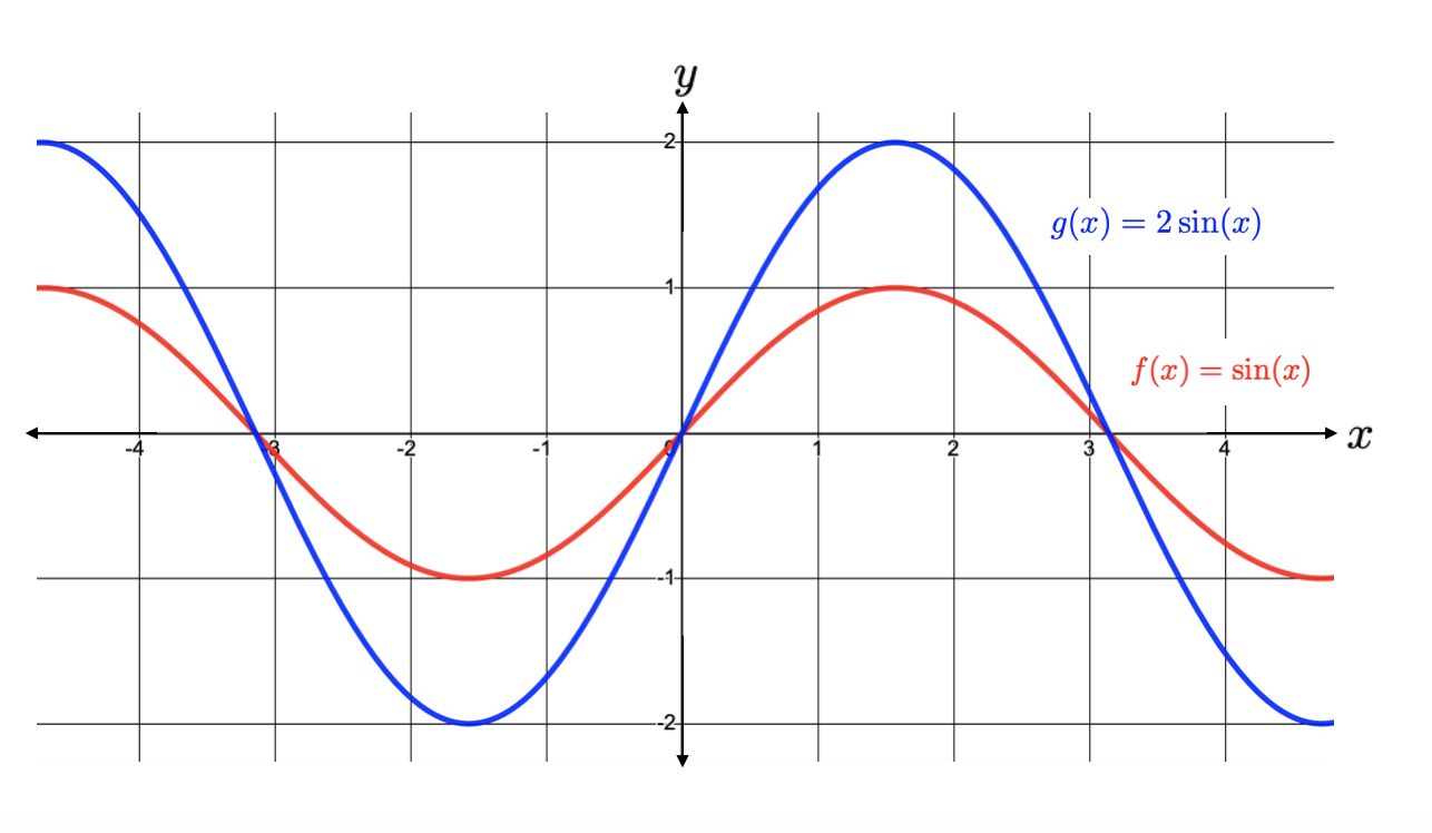
From the table, we observe that multiplying the sine function by \(2 \) results in all of the outputs of the function being multiplied by \(2\text{.}\) This results in a vertical stretch of \(\sin(x) \) by a factor of \(2\text{,}\) as seen in the graph below.
If instead we multiply the sine function by a positive number less than 1, we call this a vertical compression. For example, \(\frac{1}{3}\sin(x) \) is a vertical compression of \(\sin(x)\) by a factor of 3.
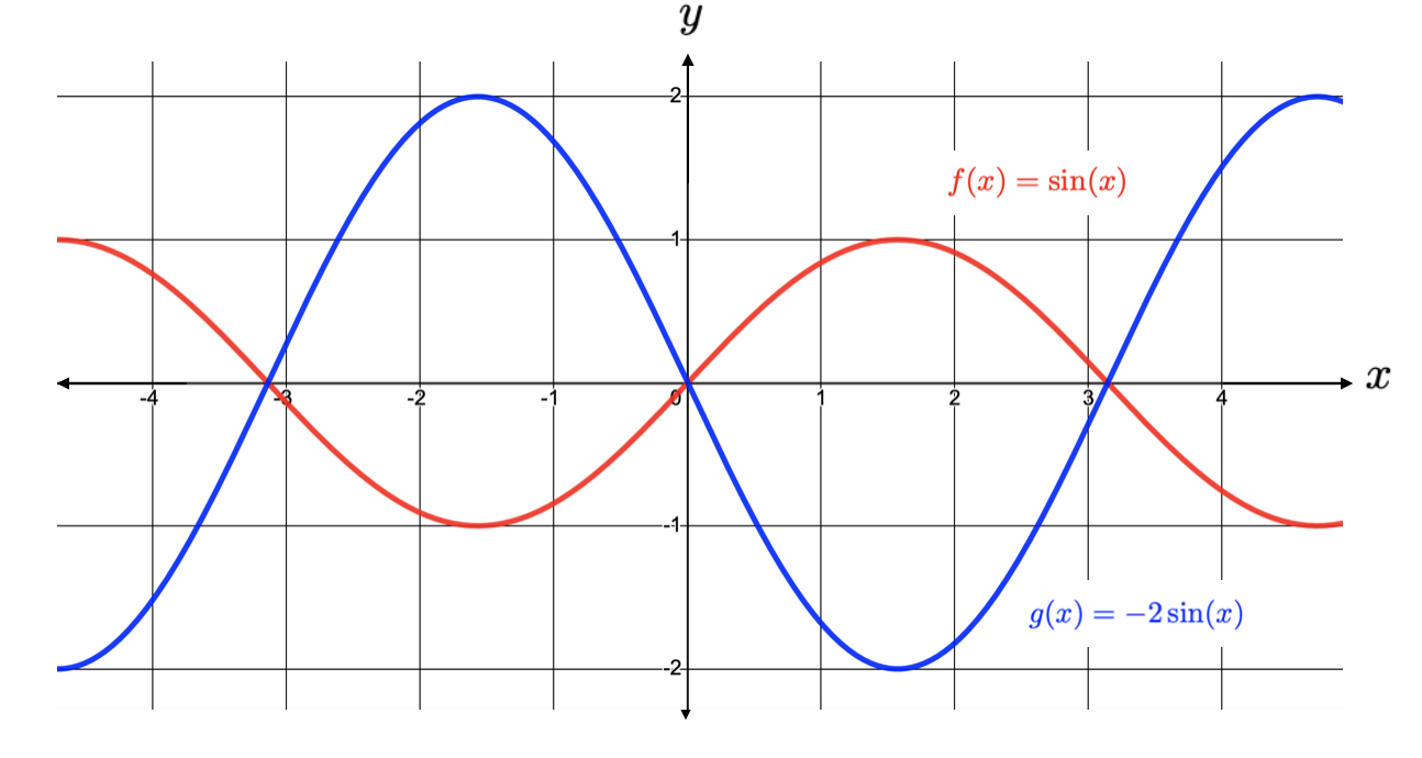
If we consider the function \(g(x) = -2\sin(x)\text{,}\) then based on our previous findings, we would expect the outputs of \(g(x)\) to be the outputs of \(\sin(x) \) multiplied by \(-2\text{.}\) This results in a vertical stretch by a factor of \(2\) and a reflection across the \(x\)-axis, as seen below:
Finally, let us consider \(g(x) =-2\sin(x)+3\text{.}\) In this case, we are multiplying the outputs of \(\sin(x)\) by \(-2\text{,}\) and then adding 3. Graphically, this results in a vertical stretch by a factor of \(2\text{,}\) a reflection across the \(x\)-axis, and finally a vertical shift up by 3 units (note that subtracting 3 would result in a shift down). We graph this below. You should verify this by creating a table like the one above.
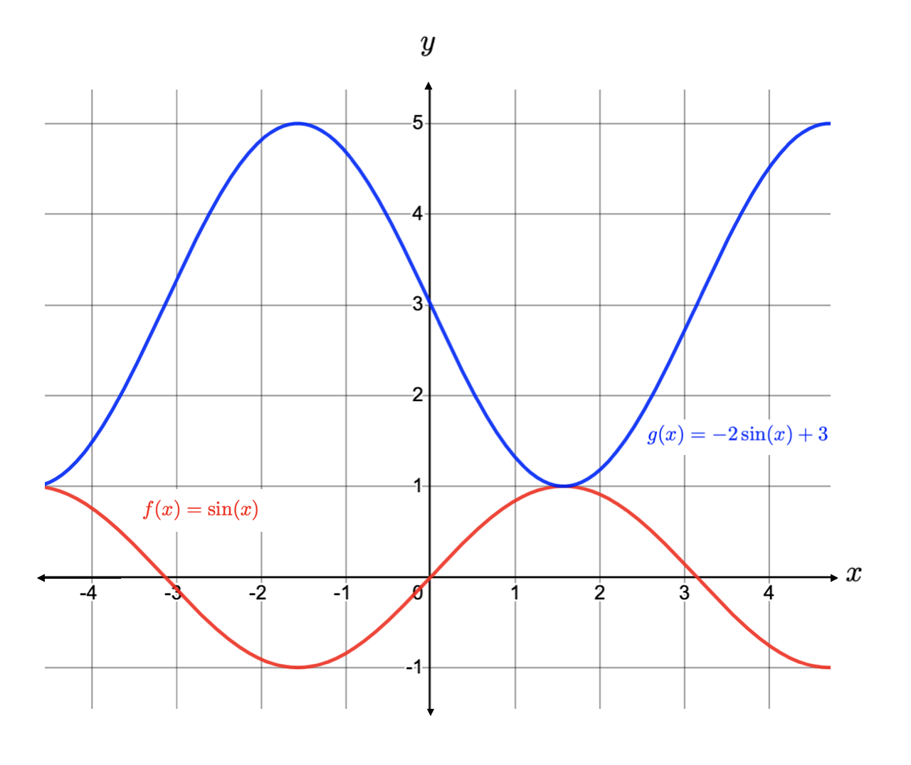
When considering the function \(g(x) =-2\sin(x)+3\) above, we multiplied the outputs of \(\sin(x)\) by -2, which resulted in a stretch and reflection, and then added 3, which resulted in a shift. This is following the order of operations (PEMDAS) and is the order that should always be used when applying vertical transformations.
Everything that we have done so far has involved \(\sin(x)\text{.}\) However, if we replace \(\sin( x)\) with any of the other trigonometric functions, we will see the same results.
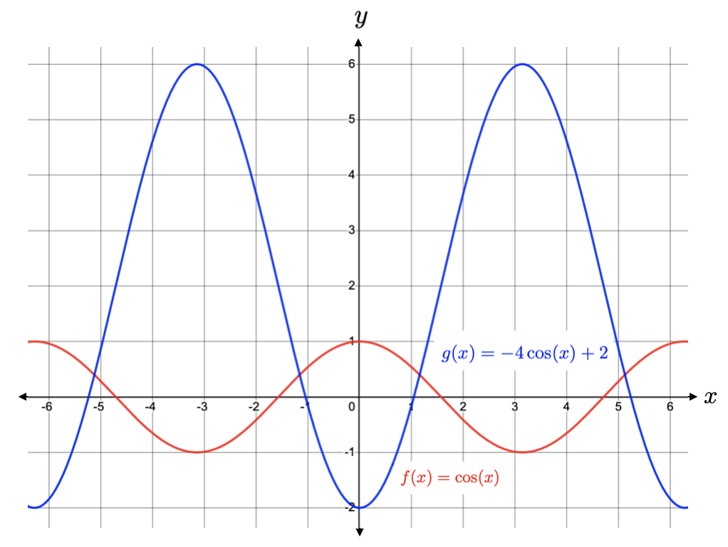
Describe how the graph of \(g(x) = -4\cos(x)+2 \) differs from the graph of \(f(x) = \cos(x) \text{.}\)
The graph of \(g(x) \) is the result of starting with the graph of \(f(x)\) and vertically stretching it by a factor of 4, then reflecting it over the \(x\)-axis, and finally shifting up by 2 units.
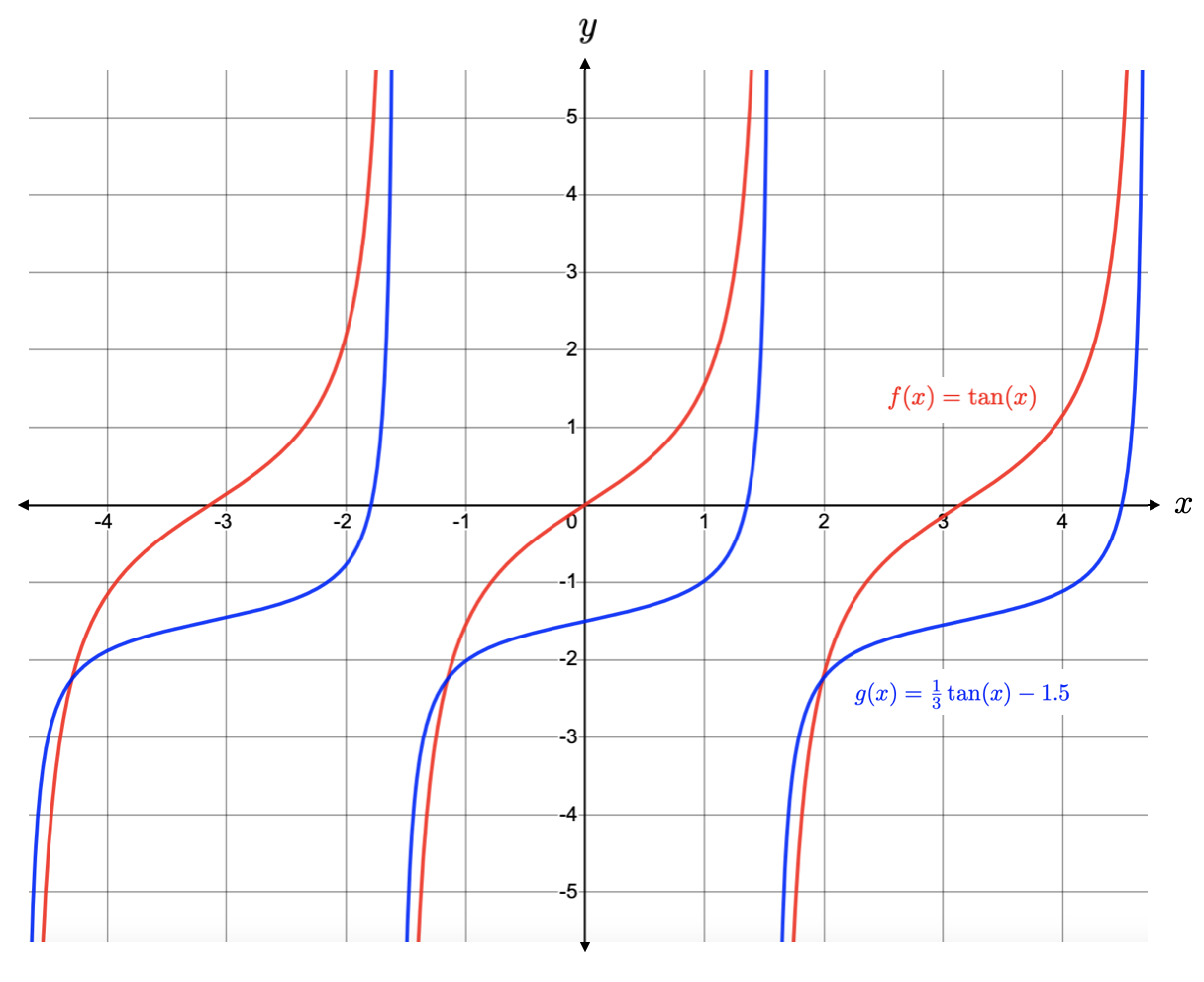
Describe how the graph of \(g(x) = \frac{1}{3}\tan(x)-1.5 \) differs from the graph of \(f(x) = \tan(x) \text{.}\)
The graph of \(g(x) \) is the result of starting with the graph of \(f(x)\text{,}\) vertically compressing it by a factor of 3, then shifting it down by 1.5 units.
Suppose we start with the graph of \(f(x) = \sin(x)\text{,}\) and we vertically stretch the graph by a factor of 3, then reflect over the \(x\)-axis, and finally shift down by 1 unit. Find the equation of the resulting function \(j(x)\text{.}\)
The equation of the resulting function is \(j(x) = -3\sin(x)-1\text{.}\)
So far we have only discussed vertical transformations, which affect the \(y\)-values of the function. Let us explore what happens when we apply horizontal transformations. Again, we will start with \(f(x) = \sin(x) \text{.}\) If we multiply the input of the function, \(x\text{,}\) by \(\pi\text{,}\) our function becomes \(g(x) = \sin(\pi x)\text{,}\) whose graph is below:
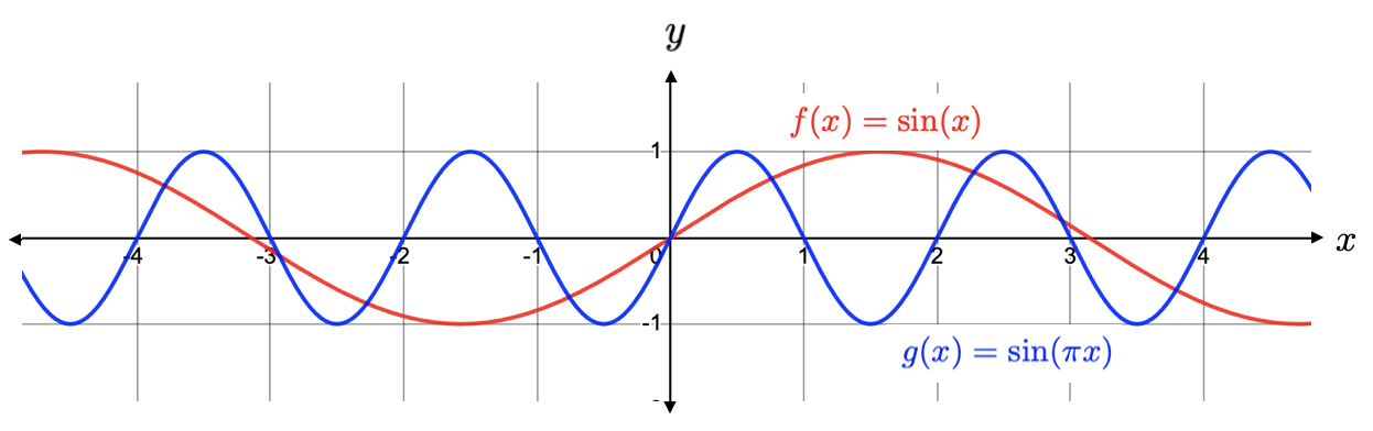
In this case, the graph of \(\sin(x) \) is horizontally compressed by a factor of \(\pi\) . If instead we multiply our input \(x\) by \(\frac{1}{\pi}\text{,}\) resulting in \(g(x) = \sin\left(\frac{1}{\pi}x\right)\text{,}\) then the graph of \(\sin(x)\) becomes horizontally stretched by a factor of \(\pi\text{.}\)
The next step here is to consider what happens if we add to or subtract from \(x\text{.}\) Consider \(g(x) = \sin\left(\pi x - \frac{\pi}{2}\right)\text{.}\) Compare the graph of \(g(x)\) with the graph of \(\sin(x)\) below:
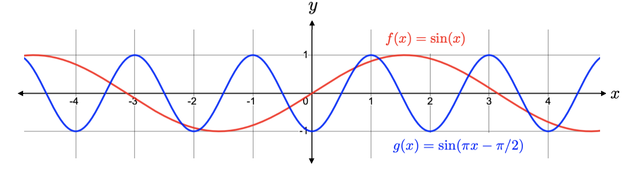
If we consider the point \((0,0)\) on the graph of \(\sin(x)\text{,}\) which is in blue, then we notice that it has shifted to the right by \(\frac{1}{2} \) units. To see where the \(\frac{1}{2}\) comes from, observe that we can rewrite \(g(x)\) as
This is really how we want to think of the function \(g(x)\text{.}\) Now, we can see that \(g(x)\) is a horizontal compression of \(\sin(x)\) by a factor of \(\pi\text{,}\) and then a horizontal shift to the right by \(\frac{1}{2}\) units. (Note that if we were to instead add \(\frac{1}{2}\text{,}\) this would result in a horizontal shift to the left by \(\frac{1}{2}\) units.)
Just like with vertical transformations, the order of horizontal transformations matters. When dealing with horizontal transformations, first be sure that the function is of the form \(g(x) = \sin(B(x-h))\text{.}\) Once it is in this form, we first horizontally stretch or compress, and then horizontally shift by \(h \) units.
Again, while everything that we have done so far has involved \(\sin(x)\text{,}\) we may apply our findings to any of the other trigonometric functions.
Suppose we have applied function transformations to \(\sin(x)\text{,}\) resulting in the function \(f(x) = A\sin(B(x-h))+k \text{.}\) The order of these transformations is:
Rewrite the function \(f(x) = \sin(3x-2)\) in the form \(f(x) = \sin(B(x-h))\text{.}\)
If we consider the form \(f(x) = \sin(B(x-h))\text{,}\) we can distribute the \(B\) over the expression \((x-h)\text{,}\) so that the function becomes \(f(x) = \sin(Bx-Bh)\text{.}\) Comparing this with \(f(x) = \sin(3x-2)\text{,}\) we see that \(B=3\) and \(Bh = 2\text{.}\) So, \(h = \frac{2}{B} = \frac{2}{3}\text{.}\) Therefore \(f(x) = \sin\left(3\left(x-\frac{2}{3}\right)\right).\) To check our answer, we can distribute the 3 inside of the sine function to get \(3\left(x-\frac{2}{3}\right) = 3x-3\cdot \frac{2}{3} = 3x-2\text{.}\)
Rewrite the function \(f(x) = 4\cos(1.5x-1)+1 \) in the form \(f(x) = A\cos(B(x-h))+k\text{.}\)
The only rewriting we need to do happens inside the cosine function with the expression \(1.5x+1\text{.}\)As in the previous example, we can identify that \(B = 1.5\text{,}\) so \(h = \frac{1}{1.5} = \frac{2}{3}\text{.}\) So, rewriting the function gives us \(f(x) = 4\cos\left(1.5\left(x-\frac{2}{3}\right)\right)\text{.}\)
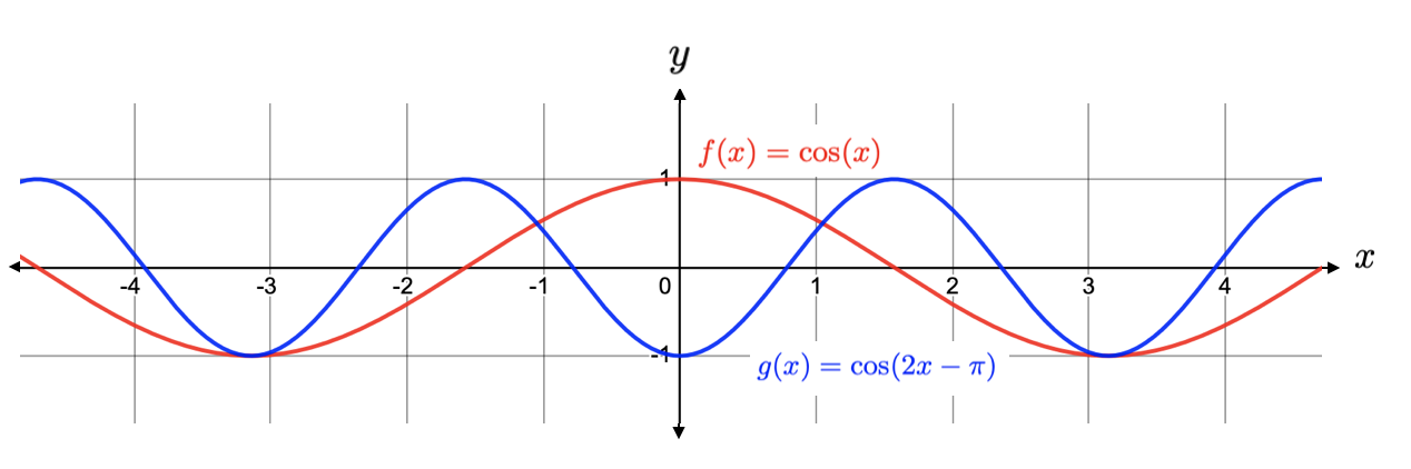
Describe how the graph of \(g(x) = \cos(2x-\pi) \) differs from the graph of \(f(x) = \cos(x) \text{.}\)
First we rewrite \(g(x)\) to be \(g(x) = \cos\left(2\left(x-\frac{\pi}{2}\right)\right). \) So, the graph of \(g(x) \) is the result of starting with the graph of \(f(x)\) and horizontally compressing it by a factor of 2 and shifting to the left by \(\frac{\pi}{2}\) units.
Suppose we start with the graph of \(f(x) = \cos(x)\text{,}\) and we horizontally stretch the graph by a factor of 2, and then shift to the left by 1 unit. Find the equation of the resulting function \(j(x)\text{.}\)
The equation of the resulting function is \(j(x) = \cos\left(\frac{1}{2}(x-1)\right)\text{.}\)
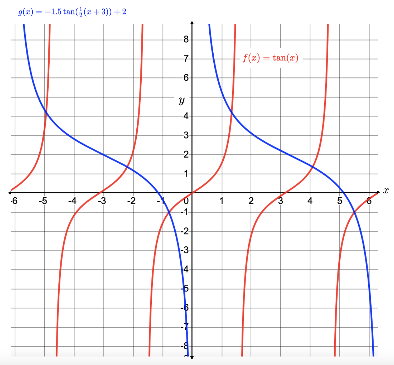
Describe how the graph of \(l(x) = -1.5\tan\left(\frac{1}{2}(x+3)\right)+2 \) differs from the graph of \(f(x) = \tan(x) \text{.}\)
Since \(l(x)\) is already in the form \(l(x) = A\tan(B(x-h))+k \text{,}\) then we do not need to rewrite it (in this case we think of the expression \((x+3)\) as \((x-(-3))\text{,}\) so \(h=-3\)).
The graph of \(l(x) \) is the result of starting with the graph of \(f(x)\text{,}\) then \(1)\) vertically stretching by a factor of 1.5, \(2)\) reflecting over the x-axis, \(3)\) vertically shifting up by 2 units, \(4)\)horizontally stretching it by a factor of 2, and finally \(5)\)then shifting it to the right by 3 units.