SectionLinear Equations
In the previous chapter, we explored algebraic expressions. In this section, we will introduce a new type of mathematical statement known as equations. In particular, we will look at linear equations and how to solve them.
In this section, you will...
define equations and what it means for an equation to be linear
solve linear equations in one variable and identify the number of solutions
manipulate linear equations in two variables
use formulas for real-world applications
Supplemental Videos
The main topics of this section are also presented in the following videos:
An equation is a mathematical statement that two expressions are equal, such as \(3x-12=0\text{.}\) A solution to an equation is any set of values that can replace the variables to produce a true statement. The variable in the equation \(3x-12=0\) is \(x\) and the solution is \(x=4\text{.}\) To verify this, substitute the value 4 in for \(x\) and check that you get a true statement:
\begin{align*}
3x-12 \amp =0\\
3(\alert{4})-12 \amp=0\\
12-12\amp =0\\
0\amp =0 \ \checkmark
\end{align*}
In this chapter, we are particularly interested in linear, or first-degree, equations. Linear equations are equations that can be written so that every term is either a constant or a constant times a single variable with no exponent. For example,
\begin{equation*}
y=-5,\: \: \: y=4x,\: \: \: 2x+4=13,\: \: \: y=14-2x,\: \: \: y=13x+9-3x
\end{equation*}
There are a few things worth noticing among these examples. First, notice that the last equation above is linear, even though it is not in its simplified form. All the terms \(13x, 9, -3x\) are either constants or constants times the variable \(x\text{.}\) If we simplify the equation, we have \(y=10x+9\text{,}\) and again, the terms \(10x\) and \(9\) are a constant times the variable and a constant, satisfying the conditions for a linear equation. Second, a linear equation can have one variable or many: \(y=-5\) is a linear equation in one variable, while \(y=4x\) is a linear equation in two variables.
Some examples of equations that are NOT linear are:
\begin{equation*}
y=x^3,\: \: \: y=-4x^2+3,\: \: \: y=3x-17+5x^3,\: \: \: y=\sqrt{x-4},\: \: \: y=\frac{1}{x}+2, \: \: \: y=2x^x
\end{equation*}
SubsectionSolving Linear Equations
To solve an equation we can generate simpler equations that have the same solutions. Equations that have identical solutions are called equivalent equations. For example,
\begin{equation*}
3x - 5 = x + 3
\end{equation*}
and
\begin{equation*}
2x = 8
\end{equation*}
are equivalent equations because the solution of each equation is \(4\text{.}\) Often we can find simpler equivalent equations by undoing in reverse order the operations performed on the variable.
By the end of this section, we will consider linear equations in more than one variable, but we will first focus on solving linear equations in a single variable.
The following list provides important rules for solving linear equations.
To Generate Equivalent Equations
We can add or subtract the same number on both sides of an equation.
We can multiply or divide both sides of an equation by the same number (except zero).
Applying either of these rules produces a new equation equivalent to the old one and thus preserves the solution. We use the rules to isolate the variable on one side of the equation.
Example43
Solve the equation \(3x - 5 = x + 3\text{.}\)
SolutionWe first collect all the variable terms on one side of the equation, and the constant terms on the other side.
\begin{align*}
3x - 5 \alert{{}- x} \amp = x + 3 \alert{{}- x}\amp\amp \text{Subtract }x \text{ from both sides.}\\
2x - 5 \amp = 3\amp\amp \text{Simplify.}\\
2x - 5 \alert{{}+ 5} \amp = 3 \alert{{}+ 5}\amp\amp \text{Add 5 to both sides.}\\
2x \amp = 8 \amp\amp\text{Simplify.}\\
\frac{2x}{\alert{2}}\amp =\frac{8}{\alert{2}}\amp\amp\text{Divide both sides by 2.}\\
x\amp = 4\amp\amp\text{Simplify.}
\end{align*}
The solution is \(4\text{.}\) (You can check the solution by substituting \(4\) into the original equation to show that you get a true statement as the result.)
The following steps should enable you to solve any linear equation. Of course, you may not need all the steps for a particular equation.
To Solve a Linear Equation
-
Simplify each side of the equation separately.
Apply the distributive law to remove parentheses.
Combine like terms.
By adding appropriate terms to both sides of the equation or subtracting appropriate terms from both sides of the equation, get all the variable terms on one side and all the constant terms on the other.
Divide both sides of the equation by the coefficient of the variable.
Example44
Solve \(3(2x - 5) - 4x = 2x - (6 - 3x)\text{.}\)
SolutionWe begin by simplifying each side of the equation.
\begin{align*}
3(2x - 5) - 4x \amp = 2x - (6 - 3x) \amp\amp\text{Apply the distributive law.}\\
6x - 15 - 4x \amp= 2x - 6 + 3x \amp\amp\text{Combine like terms on each side.}\\
2x - 15 \amp= 5x - 6
\end{align*}
Next, we collect all the variable terms on the left side of the equation, and all the constant terms on the right side.
\begin{align*}
2x - 15 \alert{- 5x} \amp= 5x - 6 \alert{- 5x} \amp\amp\text{Subtract }5x \text{ from both sides.}\\
-3x - 15 \alert{+ 15} \amp= - 6 \alert{+ 15} \amp\amp\text{Add } 15 \text{ to both sides.}\\
-3x \amp= 9
\end{align*}
Finally, we divide both sides of the equation by the coefficient of the variable.
\begin{align*}
-3x \amp= 9 \amp\amp\text{Divide both sides by }-3.\\
x \amp =-3
\end{align*}
The solution is \(-3\text{.}\)
We will often come across the need to solve linear equations with fraction or decimal coefficients. In this case, we can "clear" the denominators by multiplying both sides of the equation by the least common multiple of the denominators, as shown in the following example.
Example45
Solve \(\frac{p-2}{3}+\frac{p}{4}=\frac{1}{2}\text{.}\)
SolutionWe begin by finding the least common multiple of the three denominators: LCM\((3,4,2)=12\text{.}\) Then we multiply both sides of the equation by \(12\text{,}\) and continue solving as normal.
\begin{equation*}
\begin{aligned}
\frac{p-2}{3}+\frac{p}{4}\amp =\frac{1}{2}\\
(\alert{12})\left(\frac{p-2}{3}+\frac{p}{4}\right)\amp =(\alert{12})\frac{1}{2}\\
\frac{12(p-2)}{3}+\frac{12p}{4}\amp =\frac{12}{2}\\
4(p-2)+3p\amp =6\\
4p-8+3p\amp =6\\
7p-8\amp = 6\\
7p\amp =14\\
p\amp =2
\end{aligned}
\end{equation*}
The solution is \(p=2\text{.}\)
When we have decimal coefficients, it is sometimes easier to multiply through by \(10,100\text{,}\) etc. before solving the equation.
Example46
Solve \(0.04x+0.08x=-0.1+0.17x\text{.}\)
SolutionAs always, our first step is to combine like terms.
\begin{equation*}
\begin{aligned}
0.04x+0.08x \amp= -0.1+0.17x \\
0.12x \amp= -0.1+0.17x
\end{aligned}
\end{equation*}
Since the decimal coefficients have up to \(2\) decimal places, we will multiply each side of the equation by \(100\) before solving the equation.
\begin{equation*}
\begin{aligned}
0.12x \amp =-0.1+0.17x\\
(\alert{100})(0.12x) \amp =(\alert{100})(-0.1+0.17x)\\
2x\amp =-10+17x\\
-5x\amp =-10\\
x\amp =2
\end{aligned}
\end{equation*}
The solution is \(x=2\text{.}\)
SubsectionNumber of Solutions to Linear Equations of One Variable.
Not all linear equations have one solution. Although all of the examples above of linear equations with one variable have one solution, there are two other possible scenarios. Firstly, an equation of one variable which has equivalent expressions on both sides of the equals sign has infinitely many solutions. For example,
\begin{equation*}
3x-2 = 3x-2, \hspace{1cm} x=x, \hspace{.5cm}\text{and}\hspace{.5cm} 2(x+1) = 2x+2
\end{equation*}
all have infinitely many solutions. In this situation, any values we substitute for the variables will result in a true statement. Secondly, an equation which has two expressions that are not equal for any values of the variables has no solution. For example,
\begin{equation*}
7x+2 = 7x+10, \hspace{1cm} 17 = 0, \hspace{.5cm}\text{and}\hspace{.5cm} 2(8x+3) = 16x -5
\end{equation*}
all have no solutions. Here, no matter what values we substitute for the variables we will receive a false statement.
The number of solutions to a linear equation may not be immediately obvious. To determine the number of solutions, follow the procedures above for solving a linear equation. If at any point we have a statement which we recognize as always true or always false, then we know the equation has infinitely many or zero solutions, respectively. Else, we will finish solving the equation to determine the single solution.
Example47
Solve each equation. Determine whether there is one solution, infinitely many solutions, or no solutions.
\(5(7-2x) +1 = -10x + 25\)
\(6x = 12 - (x-7)\)
\(-36-12x = -3(12+4x)\)
Solution
-
\begin{align*}
5 (7 - 2x) +1 \amp= -10x + 25 \amp\amp \text{Apply the distributive property.}\\
35 - 10x +1 \amp= -10x + 25 \amp\amp \text{Combine like terms.}\\
-10x+36 \amp= -10x + 25
\end{align*}
Since \(-10x+36\) is not equal to \(-10x+25\) for any value of \(x\text{,}\) this equation has no solution.
-
\begin{align*}
6x\amp= 12 - (x-7) \amp\amp \text{Apply the distributive property.}\\
6x \amp= 12-x+7 \amp\amp \text{Combine like terms.}\\
6x \amp= -x+19 \amp\amp \text{Move variable terms to one side.}\\
7x \amp= 19 \amp\amp \text{Divide by coefficient on variable.}\\
x \amp=\frac{19}{7}
\end{align*}
This equation has exactly one solution, \(x=\frac{19}{7}\text{.}\)
-
\begin{align*}
-36-12x \amp= -3(12+4x) \amp\amp \text{Apply the distributive property.}\\
-36-12x \amp= -36-12x
\end{align*}
It is always the case that \(-36-12x = -36-12x\text{,}\) regardless of the value of \(x\text{.}\) In other words, this equation has infinitely many solutions.
Example48
Solve \(0.3x+1.4=-0.6x-2.2\text{.}\)
Solution
\begin{equation*}
\begin{aligned}
0.3x+1.4 \amp= -0.6x-2.2 \amp\amp\text{Multiply both sides by }10\text{ to clear the decimals.}\\
3x+14 \amp= -6x-22 \amp\amp\text{Add }6x \text{ to both sides.}\\
9x+14 \amp= -22 \amp\amp\text{Subtract }14\text{ from both sides.}\\
9x \amp= -36 \amp\amp\text{Divide both sides by 9}\\
x \amp= -4
\end{aligned}
\end{equation*}
This equation has exactly one solution, \(x=-4\text{.}\)
SubsectionLinear Equations and Formulas with Multiple Variables
Up to this point, we have only solved linear equations in one variable. Sometimes we will encounter a linear equation in more than one variable; although we cannot necessarily find an explicit solution, it may be helpful to solve such equations for particular variables.
Example49
Solve the equation \(y=3(x+8)\) for \(x\text{.}\)
SolutionTo solve for \(x\text{,}\) we can use the same processes as before: we first simplify both sides, and then isolate \(x\text{.}\)
\begin{equation*}
\begin{aligned}
y \amp= 3(x+8) \amp\amp\text{Apply the distributive property.} \\
y \amp= 3x+24 \amp\amp\text{Subtract 24 from both sides.} \\
y-24 \amp= 3x\amp\amp\text{Divide by 3.} \\
\dfrac{y-24}{3} \amp= x
\end{aligned}
\end{equation*}
Solving an equation for a given variable is particularly helpful when dealing with formulas. A formula is an equation that reflects a real-world situation. For example,
\begin{equation*}
P = 2L + 2W
\end{equation*}
gives the perimeter of a rectangle in terms of its length and width.
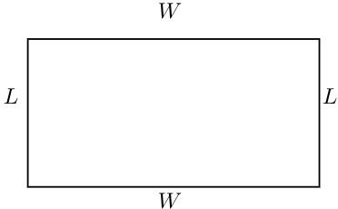
Suppose we have some wire fence to enclose an exercise area for rabbits, and we would like to see what dimensions are possible for different rectangles with that perimeter. In this case, it would be more useful to have a formula for the length of the rectangle in terms of its perimeter and its width. We can find such a formula by solving the perimeter formula for \(L\) in terms of \(P\) and \(W\text{.}\)
\begin{align*}
2L + 2W \amp= P \amp\amp\text{Subtract }2W \text{ from both sides}\\
2L \amp= P - 2W \amp\amp\text{Divide both sides by 2}\\
L \amp= \frac{P - 2W}{2}
\end{align*}
The result is a new formula that gives the length of a rectangle in terms of its perimeter and its width.
Example50
Solve \(3x - 5y = 40\) for \(y\) in terms of \(x\text{.}\)
SolutionWe isolate \(y\) on one side of the equation.
\begin{align*}
3x - 5y \amp = 40\amp\amp\text{Subtract }3x \text{ from both sides.}\\
-5y \amp = 40 - 3x\amp\amp\text{Divide both sides by }-5.\\
\frac{-5y}{-5} \amp = \frac{40 - 3x}{-5}\amp\amp\text{Simplify both sides.}\\
y \amp = -8 + \frac{3}{5}x
\end{align*}
There are many real world applications for which we can use formulas. One such useful formula is that which relates Fahrenheit to Celsius.
Example51
The formula \(5F = 9C + 160\) relates the temperature in degrees Fahrenheit, \(F\text{,}\) to the temperature in degrees Celsius, \(C\text{.}\) Solve the formula for \(C\) in terms of \(F\text{.}\)
SolutionWe begin by isolating the term that contains \(C\text{.}\)
\begin{align*}
5F \amp= 9C + 160 \amp\amp\text{Subtract 160 from both sides.}\\
5F - 160 \amp = 9C \amp\amp\text{Divide both sides by 9.}\\
\frac{5F - 160}{9} \amp =C
\end{align*}
We can also write the formula for \(C\) in terms of \(F\) as \(C = \dfrac{5}{9}F - \dfrac{160}{9}\text{.}\)
Formulas can be found in a multitude of subjects. One especially useful everyday application is that of percents. For example, simple interest \(I\) is given by the formula \(I=prt\) where \(p\) represents the principal amount invested at an annual interest rate \(r\) (as a decimal, not a percent) for \(t\) years.
Example52
Calculate the simple interest earned on a \(2\)-year investment of $\(1250\) at an annual interest rate of \(3.75\text{.}\)
SolutionWe must convert \(3.75\)% to a decimal number before using it in the formula:
\begin{equation*}
r=3.75\text{%}=0.0375
\end{equation*}
We also know that \(p=$1235\) and \(t=2\text{,}\) so
\begin{equation*}
\begin{aligned}
I\amp=prt \\ \amp=(\alert{1250})(\alert{0.0375})(\alert{2}) \\ \amp= 93.75
\end{aligned}
\end{equation*}
The simple interest earned is \($93.75\text{.}\)