MathematicsPreCalculus Mathematics at Nebraska

In the previous section we discussed the result of multiplying the output of the function by a constant value. However, what happens when we multiply the input of the function? To explore this idea, we look at the graphs of

and discuss how they are related.

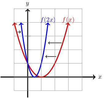
$x$	$y=f(x)$	$y=f(2x)$
$-1$	$4$	$8$
$-.5$	$2.25$	$4$
$0$	$1$	$1$
$.5$	$.25$	$0$
$1$	$0$	$1$
$2$	$1$	$9$

As we can see above, compared to the graph of $f(x)\text{,}$ the graph of $f(2x)$ is compressed horizontally by a factor of $2 \text{.}$ Effectively, if we are given a point $(x,y)$ on the graph of $f(x)$ then $\left(\dfrac{1}{2}x,y\right)$ is a point on the graph of $f(2x)\text{.}$

Looking at the table above we can verify this for a few points. For example, the point $(2,1)$ is on the graph of $f(x)\text{.}$ Then

is a point on the graph $f(2x)\text{.}$

Horizontal Stretch

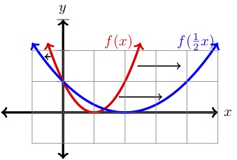
$x$	$y=f(x)$	$y=f\left(\dfrac{1}{2}x\right)$
$-1$	$4$	$2.25$
$0$	$1$	$1$
$1$	$0$	$.25$
$2$	$1$	$0$
$4$	$9$	$1$

The graph of $f\left(\dfrac{1}{2}x\right)$ is stretched horizontally by a factor of $2$ compared to the graph of $f(x) \text{.}$ Further, if $(x,y)$ is a point on the graph of $f(x)\text{,}$ then $(2x,y)$ is a point on the graph of $f\left(\dfrac{1}{2}x\right)\text{.}$

We can see this playing out in our example above. Notice that $(2,1)$ is a point on $f(x)\text{,}$ and

is a point on the graph of $f\left(\dfrac{1}{2}x\right)$ as shown in the table and graph above. In general we have:

As you may have notice by now through our examples, a horizontal stretch or compression will never change the $y$ intercepts. This is a good way to tell if such a transformation has occurred.

Example282

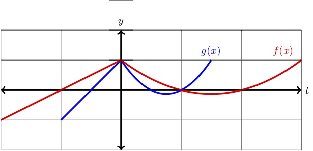
The graph of $f(x)$ is shown along with either a horizontal stretch of compression of $f(x) \text{.}$ Decide if $g(x)$ is a stretch or a compression, and give a formula for $g(x)$ in terms of $f(x)\text{.}$

Solution

First, notice that the \(y\)-intercept stays fixed while the \(x\)-intercepts shift closer to the \(y\)-axis. This tells us that \(g(x)\) is a horizontal compression. The \(x \)-intercepts of \(f(x)\) are \(x=-1,1,2 \) while the \(x\)-intercepts of \(g(x)\) are \(x=-.5,.5,1\text{.}\)

So, the \(x\)-intercepts of \(g(x) \) can be achieved by taking the intercepts of \(f(x) \) and divide each by 2. This tells us that \(g(x)\) is a horizontal compression by a factor of \(2 \text{.}\) Hence, we may write

\begin{equation*} g(x)=f(2x). \end{equation*}