In this section, you will...
generate tables to represent linear equations in two variables
graph linear equations from a table
graph lines from their equations
At the beginning of this chapter, we defined linear equations to be equations in which each term was either a constant or a constant times a single variable. In this section, we will look at linear equations in two variables, and, using the skills from the previous section, explores their graphs.
generate tables to represent linear equations in two variables
graph linear equations from a table
graph lines from their equations
The main topics of this section are also presented in the following videos:
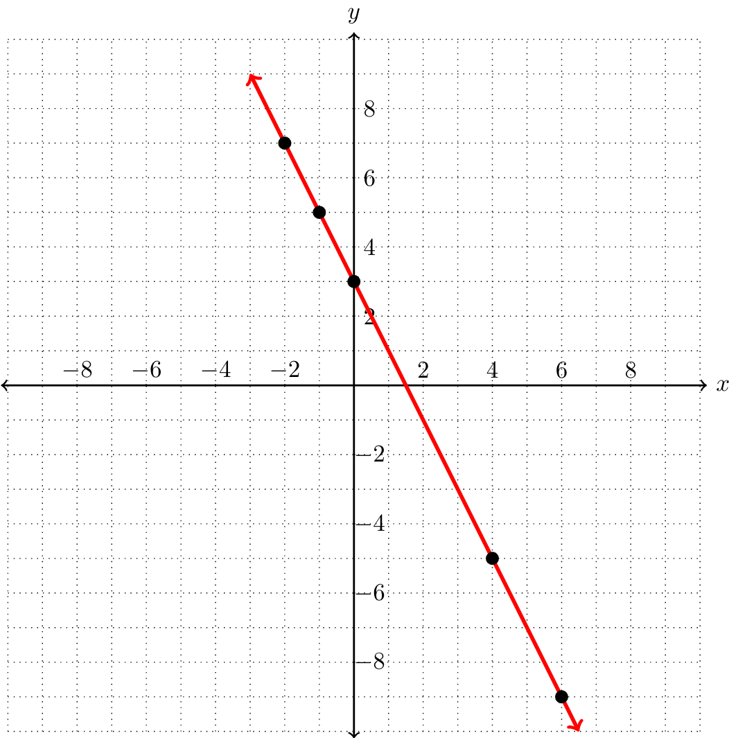
Consider the linear equation \(8x+4y=12\text{.}\) Before we try to graph this equation, let's generate a table of ordered pairs for this relation. To do so, we can pick any \(x\) values and find their corresponding \(y\) values, or vice versa. Some ordered pairs are shown below.
| \(x\) | \(y\) | Ordered pair |
| \(-2\) | \(7\) | \((-2,7)\) |
| \(-1\) | \(5\) | \((-1,5)\) |
| \(0\) | \(3\) | \((0,3)\) |
| \(4\) | \(-5\) | \((4,-5)\) |
| \(6\) | \(-9\) | \((6,-9)\) |
We can now plot these points. All of these points fall in a straight line; connecting the points, we get the graph of the equation \(8x+4y=12\text{.}\) We add arrows on either end to indicate that the graph extends indefinitely in both directions.
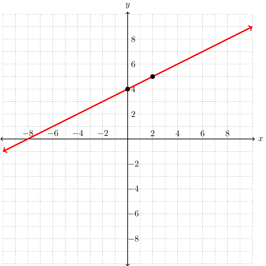
Let's create a table and graph the linear equation \(2y-x=8\text{.}\) Again, we start by generating a table with several ordered pairs that satisfy this equation.
| \(x\) | \(y\) | Ordered pair |
| \(-3\) | \(2.5\) | \((-3,2.5)\) |
| \(-1\) | \(3.5\) | \((-1,3.5)\) |
| \(0\) | \(4\) | \((0,4)\) |
| \(3\) | \(5.5\) | \((4,5.5)\) |
| \(2\) | \(5\) | \((2,5)\) |
Notice that several of the ordered pairs in our table have decimal-valued coordinates. If you are randomly selecting values of \(x\text{,}\) this will often happen and is okay. However, if you are plotting these points by hand and cannot accurately plot decimal-valued points, you should avoid using these points. In the table above, we found two points with integer coordinates: \((0,4)\) and \((2,5)\text{.}\) These two points are enough to graph this equation. We can then verify that all of the decimal-valued coordinates do in fact fall on this line.
It is often useful to describe where the graph of a linear equation meets the \(x\)- and \(y\)-axes. The point where a graph intersects the \(x\)-axis is called the \(x\)-intercept of the graph, and the point where a graph intersects the \(y\)-axis it called the \(y\)-intercept.
Look back at the graphs of \(8x+4y=12\) and \(2y-x=8\) from earlier in this section. What are the \(y\)-intercepts of each of these graphs?
The \(y\)-intercept of \(8x+4y=12\) is \((0,4)\text{.}\) The \(y\)-intercept of \(2y-x=8\) is \((0,4)\text{.}\)
It is not always clear from the graph what the intercepts of a line are. For example, consider the graph of the equation \(6y-3x=-17\text{.}\)
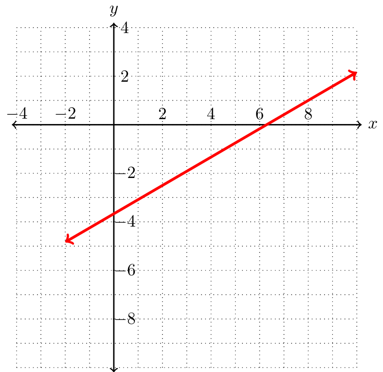
It is not clear where exactly the line is intersecting the axes. Although we could estimate where these points lie, there is a more accurate way to find the intercepts.
Think about points that lie on the \(x\)-axis. What do these points have in common? If a point lies on the \(x\)-axis, it will have the form \((x,0)\text{;}\) the \(y\)-value will always be \(0\text{.}\) This means that to find the \(x\)-intercept of a graph of a linear equation, we are looking for the \(x\)-value that corresponds to \(y=0\text{.}\) Substituting \(y=0\) into \(6y-3x=-17\text{,}\) we have
This means that the \(x\)-intercept of the graph of \(6y-3x=-17\) is \((\frac{17}{3},0)\text{.}\)
We can think about the \(y\)-intercepts similarly. Points on the \(y\)-axis have the form \((0,y)\text{,}\) so they always have \(x=0\text{.}\) To find the \(y\)-intercept of the graph of \(6y-3x=-17\text{,}\) we substitute \(x=0\text{:}\)
This means that the \(y\)-intercept of the graph of \(6y-3x=-17\) is \((0,-\frac{17}{6})\text{.}\)
Some lines don't have an \(x\)-intercept, and some lines don't have a \(y\)-intercept. Can you draw such lines? These lines will be discussed in the next section.
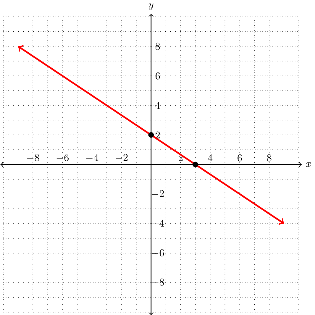
Find the \(x\)- and \(y\)-intercepts of the graph of \(6x+9y=18\text{.}\) Verify your answers by graphing the equation.
To find the \(x\)-intercept, we substitute \(y=0\text{:}\)
This means that the \(x\)-intercept is at \((3,0)\text{.}\) For the \(y\)-intercept, we substitute \(x=0\text{:}\)
Therefore the \(y\)-intercept is at \((0,2)\text{.}\)