
Supplemental Videos
The main topics of this section are also presented in the following videos:
The main topics of this section are also presented in the following videos:
Recall that in Brief Intro to Composite and Inverse Functions we gave the following definition of an inverse function:
Suppose the inverse of \(f\) is a function, denoted by \(f^{-1}\text{.}\) Then
We also stated the following property about inverse functions:
Suppose \(f^{-1}\) is the inverse function for \(f\text{.}\) Then
as long as \(x\) is in the domain of \(f\text{,}\) and \(y\) is in the domain of \(f^{-1}\text{.}\)
In this section we will explore the invertibility of a function. In other words, by the end of this section we will be able to test if a function is invertible.
In Example170, we used a graph of \(h\) to read values of \(h^{-1}\text{.}\) But we can also plot the graph of \(h^{-1}\) itself. Because \(C\) is the input variable for \(h^{-1}\text{,}\) we plot \(C\) on the horizontal axis and \(F\) on the vertical axis. To find some points on the graph of \(h^{-1}\text{,}\) we interchange the coordinates of points on the graph of \(h\text{.}\) The graph of \(h^{-1}\) is shown in Figure202.
| \(C=h(F)\) | |
| \(F\) | \(C\) |
| \(14\) | \(-10\) |
| \(32\) | \(0\) |
| \(50\) | \(10\) |
| \(68\) | \(20\) |
| \(F=h^{-1}(C)\) | |
| \(C\) | \(F\) |
| \(-10\) | \(14\) |
| \(0\) | \(32\) |
| \(10\) | \(50\) |
| \(20\) | \(68\) |

The Park Service introduced a flock of \(12\) endangered pheasant into a wildlife preserve. After \(t\) years, the population of the flock was given by
The graph of \(f\) is shown in Figure204, with \(t\) on the horizontal axis and \(P\) on the vertical axis.

The graph of \(f^{-1}\) is shown in Figure205, with \(P\) on the horizontal axis and \(t\) on the vertical axis.

The formula \(T = f(L) = 2\pi \sqrt{\dfrac{L}{32}}\) gives the period in seconds, \(T\text{,}\) of a pendulum as a function of its length in feet, \(L\text{.}\)
We can always find the inverse of a function \(y=f(x) \) simply by solving for \(x \) thus interchanging the role of the input and output variables. In the preceding examples, this process created a new function. However, this process does not always lead to be a function.
For example, to find the inverse of \(y = f (x) = x^2\text{,}\) we solve for \(x\) to get \(x = \pm\sqrt{y}\text{.}\) When we regard \(y\) as the input and \(x\) as the output, the relationship does not describe a function. This can be seen as plugging in \(y=4 \text{,}\) for example, gives two outputs \(x=2 \) and \(x=-2\text{.}\) The graphs of \(f\) and its inverse are shown in Figure207. (Note that for the graph of the inverse, we plot \(y\) on the horizontal axis and \(x\) on the vertical axis.) Because the graph of the inverse does not pass the vertical line test, it is not a function.

For many applications, it is important to know whether or not the inverse of \(f\) is a function. This can be determined from the graph of \(f\text{.}\) When we interchange the roles of the input and output variables, horizontal lines of the form \(y = k\) become vertical lines.
Thus, if the graph of the inverse is going to pass the vertical line test, the graph of the original function must pass the horizontal line test, namely, that no horizontal line should intersect the graph in more than one point. Notice that the graph of \(f(x) = x^2\) does not pass the horizontal line test, so we would not expect its inverse to be a function.
If no horizontal line intersects the graph of a function more than once, then its inverse is also a function.
We have been talking about how to tell if the inverse of a function is also a function, but in practice this is not the language typically used. Usually we ask this same question in the form "Is the function invertible?" The following definition explains this relationship: If \(y=f(x) \) is a function such that its inverse, \(x=f^{-1}(y)\text{,}\) is also a function then we say that \(f(x) \) is an invertible function.Invertible Function
Which of the functions in Figure211 are invertible?

In each case, apply the horizontal line test to determine whether the function is invertible. Because no horizontal line intersects their graphs more than once, the functions pictured in Figures211(a) and (c) are invertible. The functions in Figures211(b) and (d) are not invertibe.
The inverse function \(f^{-1}\) undoes the effect of the function \(f\text{.}\) In Example161, the function \(f(t) = 6 + 2t\) multiplies the input by \(2\) and then adds \(6\) to the result. The inverse function \(f^{-1}(H) = \dfrac{H -6}{2}\) undoes those operations in reverse order: It subtracts \(6\) from the input and then divides the result by \(2\text{.}\)
If we apply the function \(f\) to a given input value and then apply the function \(f^{-1}\) to the output from \(f\text{,}\) the end result will be the original input value. For example, if we choose \(t = 5\) as an input value, we find that \begin{align*} f(\alert{5})\amp= 6 + 2(\alert{5}) = \blert{16}\amp\amp\text{ Multiply by 2, then add 6.}\\ \text{and } f^{-1}(\blert{16}) \amp = \frac{\blert{16} - 6}{2} = \alert{5}.\amp\amp\text{Subtract 6, then divide by 2.} \end{align*}

We return to the original input value, \(5\text{,}\) as illustrated in Figure212.
Example213 illustrates the fact that if \(f^{-1}\) is the inverse function for \(f\text{,}\) then \(f\) is also the inverse function for \(f^{-1}\text{.}\)
Consider the function \(f(x) = x^3 + 2\) and its inverse, \(f^{-1}(y) = \sqrt[3]{y - 2}\text{.}\)
Example214 illustrates finding an inverse of a function. The general process is to move operations (or undo them) so the input variable (\(x\)) is what is alone on one side of the equation.
To find the inverse, we solve for \(x\text{:}\)
Therefore \(f^{-1}(y)=\frac{2}{y}+1\text{.}\)
First evaluate the function \(f\) for \(x=3\text{:}\)
Then evaluate the inverse function \(f^{-1}\) at \(y=1\text{:}\)
We started and ended with \(3\text{.}\)
First evaluate the inverse function \(f^{-1}\) for \(y=-2\text{:}\)
Then evaluate the original function \(f\) at \(x=0\text{:}\)
We started and ended with \(-2\text{.}\)
So far we have been careful to keep track of the input and output variables when we work with inverse functions. This is important when we are dealing with applications; the names of the variables are usually chosen because they have a meaning in the context of the application, and it would be confusing to change them.
However, we can also study inverse functions purely as mathematical objects. There is a relationship between the graph of a function and the graph of its inverse that is easier to see if we plot them both on the same set of axes.
A graph does not change if we change the names of the variables, so we can let \(x\) represent the input for both functions, and let \(y\) represent the output. Consider the function \(C = h(F)\) from Example170, and its inverse function, \(F = h^{-1}(C)\text{.}\) The formulas for these functions are \begin{align*} C \amp = h(F) = \frac{5}{9}(F - 32)\\ F \amp = h^{-1}(C) = 32 + \frac{9}{5}C. \end{align*} But their graphs are the same if we write them as \begin{align*} y \amp = h(x) =\frac{5}{9}(x - 32)\\ y \amp= h^{-1}(x) = 32 + \frac{9}{5}x. \end{align*} The graphs are shown in Figure215.

Now, for every point \((a, b)\) on the graph of \(f\text{,}\) the point \((b, a)\) is on the graph of the inverse function. Observe in Figure215 that the points \((a, b)\) and \((b, a)\) are always located symmetrically across the line \(y=x\text{.}\) The graphs are symmetric about the line \(y=x\), which means that if we were to place a mirror along the line \(y=x\text{,}\) each graph would be the reflection of the other.
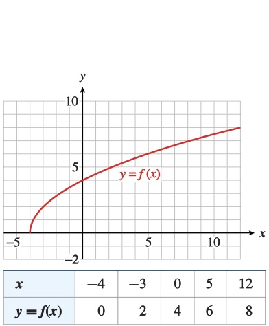
Graph the function \(f (x) = 2\sqrt{x + 4}\) on the domain \([-4, 12]\text{.}\) Graph its inverse function \(f^{-1}\) on the same grid.
The graph of \(f\) has the same shape as the graph of \(y = \sqrt{x}\text{,}\) shifted \(4\) units to the left and stretched vertically by a factor of \(2\text{.}\) Figure217a shows the graph of \(f\text{,}\) along with a table of values. By interchanging the rows of the table, we obtain points on the graph of the inverse function, shown in Figure217b.
If we use \(x\) as the input variable for both functions, and \(y\) as the output, we can graph \(f\) and \(f^{-1}\) on the same grid, as shown in Figure218. The two graphs are symmetric about the line \(y = x\text{.}\)

Graph the function \(f (x) = x^3 + 2\) and its inverse \(f^{-1}(x) = \sqrt[3]{x - 2}\) on the same set of axes, along with the line \(y = x\text{.}\)