Supplemental Videos
The main topics of this section are also presented in the following videos:
The main topics of this section are also presented in the following videos:
Many shapes, even ones as simple as circles, cannot be represented as an equation where \(y\) is a function of \(x\text{.}\) Consider, for example, the path a moon follows as it orbits around a planet, which simultaneously rotates around a sun. In some cases, equations using polar coordinates (see Section) provide a way to represent such a path. In others, we need a more versatile approach that allows us to represent both the \(x\) and \(y\) coordinates in terms of a third variable, or parameter.
A system of parametric equations is a pair of functions \(x(t)\) and \(y(t)\) in which the \(x\) and \(y\) coordinates are the output, represented in terms of a third input parameter, \(t\text{.}\)
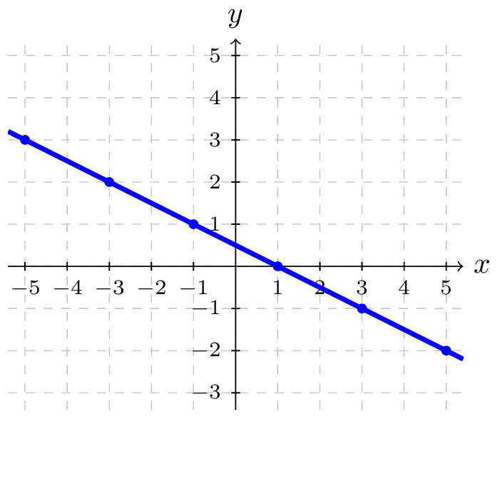
Moving at a constant speed, an object moves at a steady rate along a straight path from coordinates \((-5,3)\) to the coordinates \((3,-1)\) in \(4\) seconds, where the coordinates are measured in meters. Find parametric equations for the position of the object.
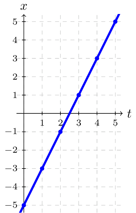
The \(x\) coordinate of the object starts at \(-5\) meters, and goes to \(+3\) meters, this means the \(x\) direction has changed by \(8\) meters in \(4\) seconds, giving us a rate of \(2\) meters per second. We can now write the \(x\) coordinate as a linear function with respect to time, \(t\text{:}\)
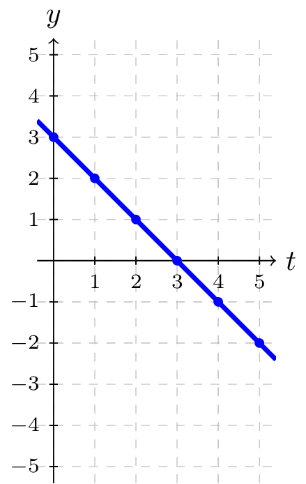
Similarly, the \(y\) value starts at \(3\) and goes to \(-1\text{,}\) giving a change in \(y\) value of \(4\) meters, meaning the \(y\) values have decreased by \(4\) meters in \(4\) seconds, for a rate of \(-1\) meter per second, giving equation \(y(t)=3-t\text{.}\)
Together, these are the parametric equations for the position of the object: \begin{align*} x(t) \amp= -5 + 2t \\ y(t) \amp= 3 - t \end{align*}
Using these equations, we can build a table of \(t\text{,}\) \(x\text{,}\) and \(y\) values. Because of the context, we limited ourselves to non-negative \(t\) values for this example, but in general you can use any values.
| \(t\) | \(x\) | \(y\) |
| \(0\) | \(-5\) | \(3\) |
| \(1\) | \(-3\) | \(2\) |
| \(2\) | \(-1\) | \(1\) |
| \(3\) | \(1\) | \(0\) |
| \(4\) | \(3\) | \(-1\) |
From this table, we could create three possible graphs: a graph of \(x\) vs. \(t\text{,}\) which would show the horizontal position over time, a graph of \(y\) vs. \(t\text{,}\) which would show the vertical position over time, or a graph of \(y\) vs. \(x\text{,}\) showing the position of the object in the plane.
There is often no single parametric representation for a curve. In Example151, we assumed the object was moving at a steady rate along a straight line. If we kept the assumption about the path (straight line) but did not assume the speed was constant, we might get a system like: \begin{align*} x(t) \amp= -5 + 2t^2 \\ y(t) \amp= 3 - t^2 \end{align*}
You can explore this in a tool like Desmos, and you'll find that although the separate graphs for \(x(t)\) and \(y(t)\) are not themselves linear, graphing \(x\) vs. \(y\) does indeed give a straight-line path, exactly the same one as in Example151!
In Section, we explored how the unit circle can be described as the collection of all \((x,y)\)-coordinates that satisfy the equation
It is not possible to rewrite this in a form \(y=f(x)\text{.}\) The best we can do is express just the top half of the circle in the form \(y=f(x)\text{,}\) or just the bottom half of the circle, as depicted in Figure156.
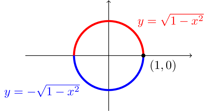
If we could write down an expression for the unit circle in a form \(y=f(x)\text{,}\) it would be convenient for graphing. We could build a table of \((x,y)\)-coordinates by plugging various \(x\) values into the function \(f(x)\) and finding corresponding \(y\) values, then draw a graph based on the table of values.
However, Example151 above shows how one can still draw a graph by building a table of \((x,y)\)-coordinate values using parametric equations (by plugging in various values for \(t\) into each equation for the \(x\)- and \(y\)-coordinates). Throughout this section, we'll see many examples of shapes for which \(y\) is not a function of \(x\text{,}\) but we can describe their graphs using parametric equations.
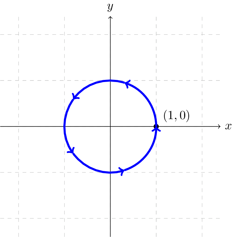
Sketch a graph of \begin{align*} x(t) \amp= \cos(t) \\ y(t) \amp= \sin(t) \end{align*}
These equations should look familiar. Back when we first learned about sine and cosine we found that the coordinates of a point on the unit circle at an angle of \(\theta\) will be \(x=\cos\theta\text{,}\) \(y=\sin\theta\text{.}\) The equations above are in the same form with \(t\) used in place of \(\theta\text{.}\)
This suggests that for each value of \(t\text{,}\) these parametric equations give a point on the unit circle at the angle corresponding to \(t\text{.}\) At \(t=0\text{,}\) the graph would be at \(x=\cos(0)\text{,}\) \(y=\sin(0)\text{,}\) the point \((1,0)\text{.}\) Indeed, these equations describe the equation of the unit circle, drawn counterclockwise.
Interestingly, these similar parametric equations also describe the unit circle: \begin{align*} x(t) \amp= \sin(t) \\ y(t) \amp= \cos(t) \end{align*}
The difference with these equations is the graph would start at \(x=\sin(0)\text{,}\) \(y=\cos(0)\text{,}\) the point \((0,1)\text{.}\) As \(t\) increases from \(0\text{,}\) the \(x\) value will increase, indicating these equations would draw the graph in a clockwise direction.
In Section, we reviewed the rules for how changes to formulae (of the form \(y=f(x)\)) are related to transformations of graphs of functions. With parametric equations, although we may not be able to represent a curve in a form \(y=f(x)\text{,}\) we'll find that it is very intuitive to adjust our parametric equations for standard transformations of functions.
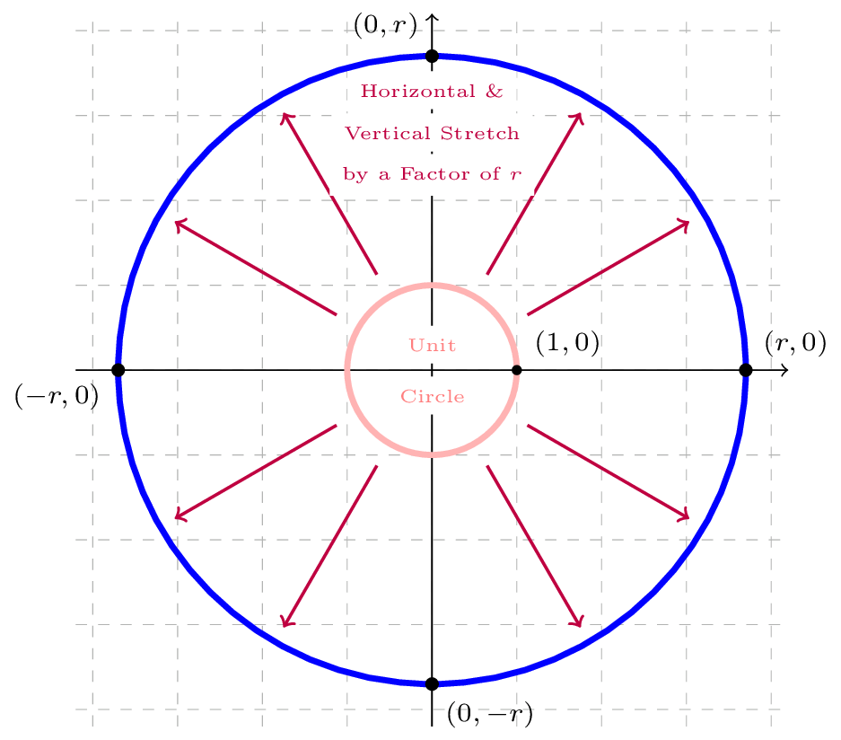
Let's start by considering a simultaneous vertical and horizontal stretch by a factor of \(r\text{,}\) which when applied to the unit circle, actually results in a circle of radius \(r\) centered at the origin (see Figure158).
Example157 showed that the following set of parametric equations represents the unit circle: \begin{align*} x(t) \amp= \cos(t) \\ y(t) \amp= \sin(t) \end{align*}
This was determined because the functions cosine and sine give the \(x\)- and \(y\)-coordinates, respectively, of points on the unit circle. Although we're slightly more used to thinking about how \(\cos\theta\) and \(\sin\theta\) are related to points on the unit circle, it is a standard practice to use the variable \(t\) in parametric equations, so as \(t\) increases, we think of the angle at the origin measured from the positive \(x\)-axis increasing (and therefore, the circle is drawn counterclockwise as \(t\) increases in the parametric equations.
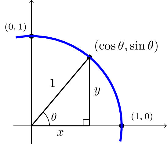
Figure159 shows how the \(x\)- and \(y\)-coordinates of a point on the circle of radius \(r\) centered at the origin relate to the angle measured from the positive \(x\)-axis. We label this angle \(t\) right away, since it will be used in a set of parametric equations.
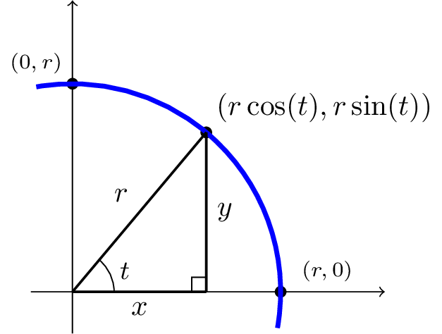
The coordinates expressed in terms of \(r\) and \(t\) come from the following relationships relating to the right triangle drawn in Figure159:
For example, the first relationship tells us that \(\cos(t)=\frac{x}{r}\text{,}\) so multiplying both sides by \(r\) gives \(x=r\cos(t)\text{.}\)
Therefore, we have a way to represent the \(x\)- and \(y\)-coordinates of points on the circle of radius \(r\) centered at the origin in terms of the variable \(t\text{,}\) giving us the following set of parametric equations: \begin{align*} x(t) \amp= r \cos(t) \\ y(t) \amp= r \sin(t) \end{align*}
Let's add one more type of transformation before we formalize this result.
A circle not centered at the origin can be obtained by starting with a circle centered at the origin (of the same radius) and shifting it horizontally some number of units, then vertically some number of units. See Section for a detailed example of obtaining a circle not centered at the origin as a result of these types of shifts.
Suppose we wish to describe a circle of radius \(r\) centered at the point \((h,k)\text{.}\) First, from our previous work, we know that the circle of radius \(r\) which is centered at the origin can be described by the following parametric equations: \begin{align*} x(t) \amp= r \cos(t) \\ y(t) \amp= r \sin(t) \end{align*}
The circle centered at the point \((h,k)\) can be thought of as the result of shifting the circle centered at the origin. Here, we'll build parametric equations to describe this circle of the following form (where we are using capital letter just to help distinguish from other parametric equations in this section): \begin{align*} X(t) \amp= \underline{\;\;\;\;\;\;\;\;\;\;\;\;\;\;\;\;} \\ Y(t) \amp= \underline{\;\;\;\;\;\;\;\;\;\;\;\;\;\;\;\;} \end{align*}
First, the \(x\)-coordinate of the center of the circle is now \(h\) instead of \(0\text{,}\) which means that we need to shift the circle horizontally by \(h\) units, or equivalently, we need to add \(h\) units to the \(x\)-coordinate of each point on the circle centered at the origin. With parametric equations, the \(x\)-coordinates have their very own equation, so it is actually very convenient to isolate and adjust exactly what we need with the \(x\)-coordinates to build \(X(t)\text{:}\)
Similarly, we may obtain a formula for the \(y\)-coordinates of the circle centered at \((h,k)\) by realizing they are related to the \(y(t)\text{,}\) the \(y\)-coordinates of the circle centered at the origin, but shifted by \(k\) units:
In summary, we have a nice general way of building parametric equations to describe any circle in the plane:
A circle of radius \(r\) centered at the point \((h,k)\) can be described using the following pair of parametric equations: \begin{align*} x(t) \amp= r \cos(t) + h \\ y(t) \amp= r \sin(t) + k \end{align*}
Recall from Section that we can describe an ellipse as being a circle which is stretched both horizontally and vertically, but not by the same stretch factor. Our goal in this section is to come up with a set of parametric equations that can describe a general ellipse.
Above, we build parametric equations for a circle of radius \(r\) by multiplying both the \(x\)- and \(y\)-coordinate functions by a factor of \(r\text{,}\) thus stretching the circle uniformly by a factor of \(r\) both horizontally and vertically.
Suppose instead that we wish to obtain an ellipse that, compared to the unit circle, has been stretched by a factor of \(5\) in the horizontal direction and by a factor of \(3\) in the vertical direction. The parametric equations that describe this ellipse will have the following form: \begin{align*} X(t) \amp= \underline{\;\;\;\;\;\;\;\;\;\;\;\;\;\;\;\;} \\ Y(t) \amp= \underline{\;\;\;\;\;\;\;\;\;\;\;\;\;\;\;\;} \end{align*} Let's start with parametric equations for the unit circle: \begin{align*} x(t) \amp= \cos(t) \\ y(t) \amp= \sin(t) \end{align*}
First, let's consider what happens when we stretch the unit circle horizontally by a factor of \(5\text{.}\) In doing just this, we wish to adjust the \(x\)-coordinates of points on the graph while leaving the \(y\)-coordinates unchanged. Again, with parametric equations, the \(x\)- and \(y\)-coordinates are isolated into separate equations, so it is convenient to stretch out only the \(x\)-coordinates by a factor of \(5\text{:}\)
Similarly, we can define \(Y(t)\) to represent a vertical stretch by a factor of \(3\text{,}\) adjusting only the \(y\)-coordinates:
The following set of parametric equations is therefore the result of stretching the unit circle horizontally by a factor of \(5\) and vertically by a factor of \(3\text{,}\) giving a set of parametric equations to describe the ellipse as desired: \begin{align*} X(t) \amp= 5 \cos(t) \\ Y(t) \amp= 3 \sin(t) \end{align*}
We generalize this reasoning with the following important result for defining parametric equations for ellipses, along with an adjustment for shifting the center of the ellipse as well:
An ellipse centered at the point \((h,k)\) can be described using the following pair of parametric equations: \begin{align*} x(t) \amp= a \cos(t) + h \\ y(t) \amp= b \sin(t) + k \end{align*} where the ellipse is obtained by stretching the unit circle by a factor of \(a\) in the horizontal direction and a factor of \(b\) in the vertical direction.
A light is placed on the edge of a bicycle tire as shown and the bicycle starts rolling down the street. Find a parametric equation for the position of the light after the wheel has rotated through an angle of \(\text{.}\)
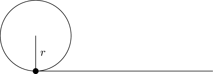
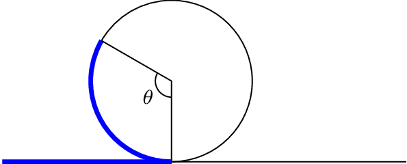
Relative to the center of the wheel, the position of the light can be found as the coordinates of a point on a circle, but since the \(x\) coordinate begins at \(0\) and moves in the negative direction, while the \(y\) coordinate starts at the lowest value, the coordinates of the point will be given by: \begin{align*} x \amp= -r \sin\theta \\ y \amp= -r \cos\theta \end{align*}
The center of the wheel, meanwhile, is moving horizontally. It remains at a constant height of \(r\text{,}\) but the horizontal position will move a distance equivalent to the arc length of the circle drawn out by the angle, \(s=r\theta\text{.}\) The position of the center of the circle is then \begin{align*} x \amp= r \theta \\ y \amp= r \end{align*}
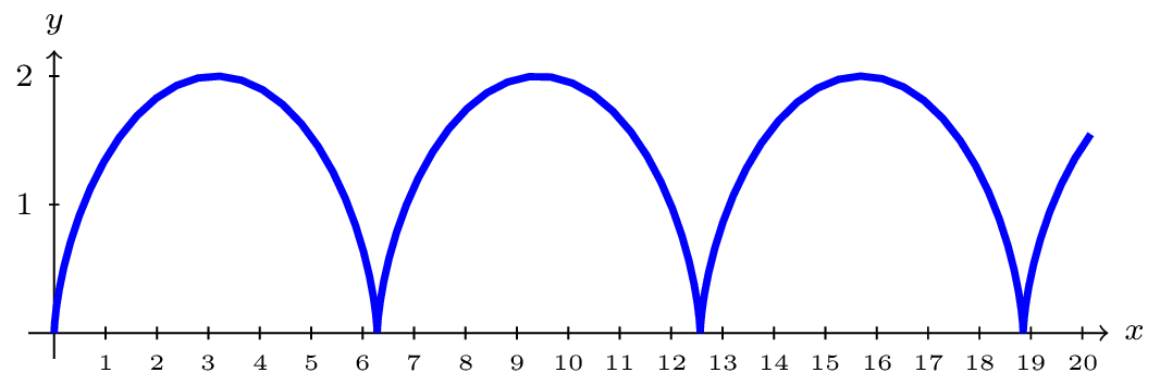
Combining the position of the center of the wheel with the position of the light on the wheel relative to the center, we get the following parametric equations, with \(\theta\) as the parameter: \begin{align*} x \amp= r \theta - r \sin\theta = r (\theta-\sin\theta) \\ y \amp= r - r \cos\theta = r (1-\cos\theta) \end{align*}
The result graph is called a cycloid.
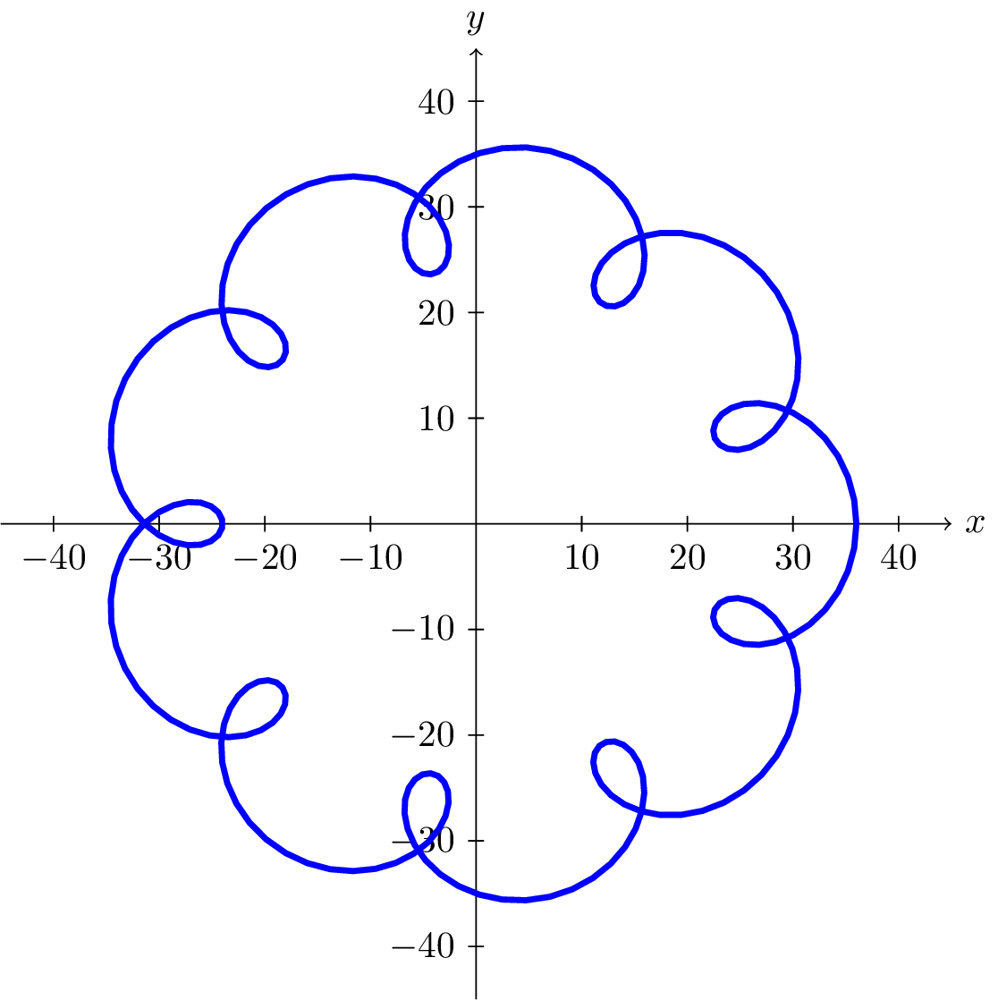
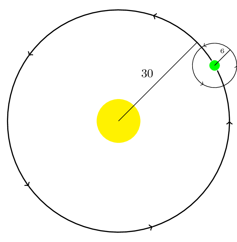
A moon travels around a planet as shown, orbiting once every \(10\) days. The planet travels around a sun as shown, orbiting once every \(100\) days. Find a parametric equation for the position of the moon, relative to the center of the sun, after \(t\) days.
For this example, we'll assume the orbits are circular, though in real life they're actually elliptical.
The coordinates of a point on a circle can always be written in the form \begin{align*} x \amp= r \cos\theta \\ y \amp= r \sin\theta \end{align*}
Since the orbit of the moon around the planet has a period of \(10\) days, the equation for the position of the moon relative to the planet will be \begin{align*} x(t) \amp= 6 \cos \left( \frac{2\pi}{10} t \right) = 6 \cos \left( \frac{\pi}{5} t \right) \\ y(t) \amp= 6 \sin \left( \frac{2\pi}{10} t \right) = 6 \sin \left( \frac{\pi}{5} t \right) \\ \end{align*}
With a period of \(100\) days, the equation for the position of the planet relative to the sun will be \begin{align*} x(t) \amp= 30 \cos \left( \frac{2\pi}{100} t \right) = 30 \cos \left( \frac{\pi}{50} t \right) \\ y(t) \amp= 30 \sin \left( \frac{2\pi}{100} t \right) = 30 \sin \left( \frac{\pi}{50} t \right) \\ \end{align*}
Combining these together, we can find the position of the moon relative to the sun as the sum of the components. \begin{align*} x(t) \amp= 6 \cos \left( \frac{\pi}{5} t \right) + 30 \cos \left( \frac{\pi}{50} t \right) \\ y(t) \amp= 6 \sin \left( \frac{\pi}{5} t \right) + 30 \sin \left( \frac{\pi}{50} t \right) \\ \end{align*}
The resulting graph is shown here.