Supplemental Videos
The main topics of this section are also presented in the following videos:
The main topics of this section are also presented in the following videos:
Most people have intuition about what is means for something to be increasing and what it means for something to be decreasing. However, we need to develop a solid mathematical way of defining increasing and decreasing.
Before defining increasing and decreasing is will be useful to recall interval notation.
An interval is a set that consists of all the real numbers between two numbers \(a\) and \(b\text{.}\)
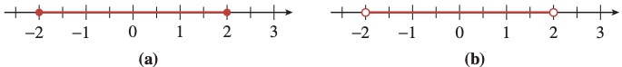
The set \(-2 \le x \le 2\) includes its endpoints \(-2\) and \(2\text{,}\) so we call it a closed interval, and we denote it by \([-2, 2]\) (see Figure56a). The square brackets tell us that the endpoints are included in the interval. An interval that does not include its endpoints, such as \(-2 \lt x \lt 2\text{,}\) is called an open interval, and we denote it with round brackets, \((-2, 2)\) (see Figure56b).
Do not confuse the open interval \((-2, 2)\) with the point \((-2, 2)\text{!}\) The notation is the same, so you must decide from the context whether an interval or a point is being discussed.
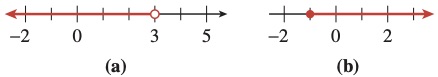
We can also discuss infinite intervals, such as \(x\lt 3\) and \(x\ge -1\text{,}\) shown in Figure58. We denote the interval \(x\lt 3\) by \((-\infty, 3)\text{,}\) and the interval \(x\ge -1\) by \([-1, \infty)\text{.}\) The symbol \(\infty\text{,}\) for infinity, does not represent a specific real number but rather indicates that the interval continues forever along the real line. Because of this, we will always use a round bracket along side \(\pm \infty\text{.}\)
Some intervals are closed on one end and open on the other. We call such an interval a half-open or half-closed interval. Some examples of half-open/half-closed intervals are \([-2,9)\) and \((0,23]\text{.}\)
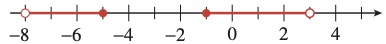
Finally, we can combine two or more intervals into a larger set. For example, the set consisting of \(x\lt -1\) or \(x\gt 2\text{,}\) shown in Figure59, is the union of two intervals and is denoted by \((-\infty,-2) \cup (2,\infty)\text{.}\)

Many solutions of inequalities are intervals or unions of intervals.
Write each of the solution sets with interval notation and graph the solution set on a number line.
\(3 \le x \lt 6\)
\(x \ge -9\)
\(x\le 1 ~\text{ or }~ x\gt 4\)
\(-8 \lt x \le -5 ~\text{ or }~ -1 \le x \lt 3\)
\([3, 6)\text{.}\) (See Figure61.)

\([-9,\infty)\text{.}\) We always use round brackets next to the symbol \(\infty\) because \(\infty\) is not a specific number and is not included in the set. (See Figure62.)

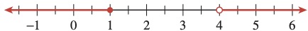
\((-\infty, 1] \cup (4, \infty)\text{.}\) The word or describes the union of two sets. (See Figure63.)
\((-8,-5] \cup [-1, 3)\text{.}\) (See Figure64.)
Now that we have reviewed interval notation we are positioned to define increasing and decreasing functions
Let \(y = f(x)\) where \(a\leq x \leq b.\)
Then the function \(f(x)\) is said to be increasing on \((a,b)\) if the value of \(f(x)\) increases as \(x\) increases on \((a,b)\text{.}\)
Then the function \(f(x)\) is said to be decreasing on \((a,b)\) if the value of \(f(x)\) decreases as \(x\) increases on \((a,b)\text{.}\)
If the graph of a function has arrows on the ends then we can assume that the function continues in that same general direction.
On what intervals is the function graphed in Figure88 decreasing?
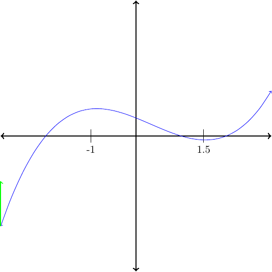
The function is decreasing on the intervas \((-1,1.5)\text{.}\)
Imagine you are an ant carrying a heavy burden along one of the two paths shown in Figure89. Which path is more difficult? Most ants would agree that the steeper path is more difficult.
But what exactly is steepness? It is not merely the gain in altitude, because even a gentle incline will reach a great height eventually. Steepness measures how sharply the altitude increases. An ant finds the second path more difficult, or steeper, because it rises 5 feet while the first path rises only 2 feet over the same horizontal distance.

To compare the steepness of two inclined paths, we compute the ratio of change in altitude to change in horizontal distance for each path.
Which is steeper, Stony Point trail, which climbs 400 feet over a horizontal distance of 2500 feet, or Lone Pine trail, which climbs 360 feet over a horizontal distance of 1800 feet?
For each trail, we compute the ratio of vertical gain to horizontal distance. For Stony Point trail, the ratio is
and for Lone Pine trail, the ratio is
Lone Pine trail is steeper, because it has a vertical gain of 0.20 foot for every foot traveled horizontally. Or, in more practical units, Lone Pine trail rises 20 feet for every 100 feet of horizontal distance, whereas Stony Point trail rises only 16 feet over a horizontal distance of 100 feet.
To compare the steepness of the two trails in Example90, it is not enough to know which trail has the greater gain in elevation overall. Instead, we compare their elevation gains over the same horizontal distance. Using the same horizontal distance provides a basis for comparison. The two trails are illustrated in Figure92 as lines on a coordinate grid.

The ratio we computed in Example90,
appears on the graphs in Figure92 as
For example, as we travel along the line representing Stony Point trail, we move from the point \((0, 0)\) to the point \((2500, 400)\text{.}\) The \(y\)-coordinate changes by \(400\) and the \(x\)-coordinate changes by \(2500\text{,}\) giving the ratio \(0.16\) that we found in Example90. We call this ratio the slope of the line.
The slope of a line is the ratio
as we move from one point to another on the line.
Compute the slope of the line that passes through points \(A\) and \(B\) in Figure94.

As we move along the line from \(A\) to \(B\text{,}\) the \(y\)-coordinate changes by \(3\) units, and the \(x\)-coordinate changes by \(4\) units. The slope of the line is thus
Compute the slope of the line through the indicated points in Figure96. On both axes, one square represents one unit.

\(m=\dfrac{2}{8}=\dfrac{1}{4} \)
The slope of a line is a number. It tells us how much the \(y\)-coordinates of points on the line increase when we increase their \(x\)-coordinates by 1 unit. For instance, the slope \(\dfrac{3}{4}\) in Example93 means that the \(y\)-coordinate increases by \(\dfrac{3}{4}\) unit when the \(x\)-coordinate increases by 1 unit. For increasing graphs, a larger slope indicates a greater increase in altitude, and hence a steeper line.
We use a shorthand notation for the ratio that defines slope,
The symbol \(\Delta\) (the Greek letter delta) is used in mathematics to denote change in. In particular, \(\Delta y\) means change in \(y\)-coordinate, and \(\Delta x\) means change in \(x\)-coordinate. We also use the letter \(m\) to stand for slope. With these symbols, we can write the definition of slope as follows.
The slope of a line is given by

The Great Pyramid of Khufu in Egypt was built around 2550 B.C. It is 147 meters tall and has a square base 229 meters on each side. Calculate the slope of the sides of the pyramid, rounded to two decimal places.
The Kukulcan Pyramid at Chichen Itza in Mexico was built around 800 A.D. It is \(24\) meters high, with a temple built on its top platform, as shown in Figure100.
The square base is \(55\) meters on each side, and the top platform is \(19.5\) meters on each side. Calculate the slope of the sides of the pyramid. Which pyramid is steeper, Kukulcan or the Great Pyramid?

The slope of the sides of the Kukulcan Pyramid is \(\frac{24}{17.5}\text{,}\) which is approximately \(1.35\text{;}\) Kukulcan is steeper.
So far, we have only considered examples in which \(\Delta x\) and \(\Delta y\) are positive numbers, but they can also be negative.
Compute the slope of the line that passes through the points \((-4, 2)\) and \((5, -1)\) shown in Figure102 Illustrate \(\Delta y\) and \(\Delta x\) on the graph.
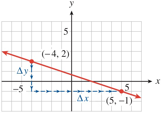
As we move from the point \((-4, 2)\) to the point \((5, -1)\text{,}\) we move \(3\) units down, so \(\Delta y = -3\text{.}\) We then move \(9\) units to the right, so \(\Delta x = 9\text{.}\) Thus, the slope is
\(\Delta y\) and \(\Delta x\) are labeled on the graph.
We can move from point to point in either direction to compute the slope. The line graphed in Example101 decreases as we move from left to right and hence has a negative slope.
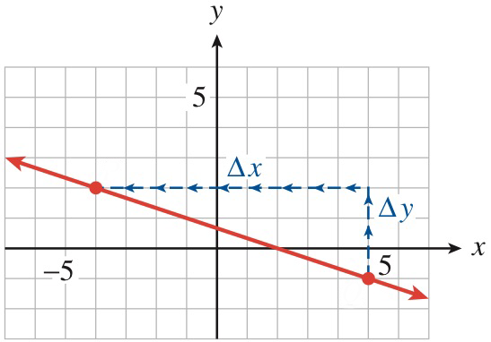
The slope is the same if we move from point \((5,-1)\) to point \((-4,2)\) instead of from \((-4,2)\) to \((5,-1)\text{.}\) (See Figure103.) In that case, our computation looks like this:
\(\Delta y\) and \(\Delta x\) are labeled on the graph.
How do we know which two points to choose when we want to compute the slope of a line? It turns out that any two points on the line will do.
Graph the line \(4x - 2y = 8\) by finding the \(x\)- and \(y\)-intercepts
Compute the slope of the line using the \(x\)-intercept and \(y\)-intercept.
Compute the slope of the line using the points \((4, 4)\) and \((1, -2)\text{.}\)

\(2\)
\(2\)
Example104 illustrates an important property of lines: They have constant slope. No matter which two points we use to calculate the slope, we will always get the same result. We will see later that lines are the only graphs that have this property.
We can think of the slope as a scale factor that tells us how many units \(y\) increases (or decreases) for each unit of increase in \(x\text{.}\) Compare the lines in Figure106

Observe that a line with positive slope increases from left to right, and one with negative slope decreases. What sort of line has slope \(m = 0\text{?}\)
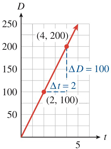
Consider the graph of the equation \(C = 5 + 3t\) showing the cost of a bicycle rental in terms of the length of the rental. Figure107 We can choose any two points on the line to compute its slope. Using points \(P\) and \(Q\) as shown, we find that
The slope of the line is \(3\text{.}\)

What does this value mean for the cost of renting a bicycle? The expression
stands for
If we increase the length of the rental by 3 hours, the cost of the rental increases by 9 dollars. The slope gives the rate of increase in the rental fee, 3 dollars per hour. In general, we can make the following statement.
The slope of a line measures the rate of change of the output variable with respect to the input variable.
Depending on the variables involved, this rate might be interpreted as a rate of growth or a rate of speed. A negative slope might represent a rate of decrease or a rate of consumption. The slope of a graph can give us valuable information about the variables.
The graph in Figure109 shows the distance in miles traveled by a big-rig truck driver after \(t\) hours on the road.
The graph in Figure111 shows the altitude, \(a\) (in feet), of a skier \(t\) minutes after getting on a ski lift.
Choose two points and compute the slope (including units).
What does the slope tell us about the problem?

\(150\)
Altitude increases by \(150\) feet per minute.
We have defined the slope of a line to be the ratio \(m = \dfrac{\Delta y}{\Delta x}\) as we move from one point to another on the line. So far, we have computed \(\Delta y\) and \(\Delta x\) by counting squares on the graph, but this method is not always practical. All we really need are the coordinates of two points on the graph.
We will use subscripts to distinguish the two points: let \((x_1, y_1)\) be the coordinates of the first points and let \((x_2, y_2)\) be the coordinates of the second point.
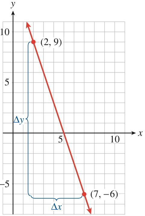
Now consider a specific example. The line through the two points \((2, 9)\) and \((7,-6)\) is shown in Figure112. We can find \(\Delta x\) by subtracting the \(x\)-coordinates of the points:
In general, we have
and similarly
These formulas work even if some of the coordinates are negative; in our example,
By counting squares down from \((2,9)\) to \((7,-6)\text{,}\) we see that \(\Delta y\) is indeed \(-15\text{.}\) The slope of the line in Figure112 is
\begin{align*} m\amp=\frac{\Delta y}{\Delta x}=\frac{y_2 - y_1}{x_2 - x_1} \\ \amp=\frac{-15}{5} = -3. \end{align*}
We now have a formula for the slope of a line that works even if we do not have a graph.
The slope of the line passing through the points \((x_1, y_1)\) and \((x_2, y_2)\) is given by
Compute the slope of the line in Figure112 using the points \((6, -3)\) and \((4, 3)\text{.}\)
Substitute the coordinates of \((6, -3)\) and \((4, 3)\) into the slope formula to find
This value for the slope, \(-3\text{,}\) is the same value found above.
Find the slope of the line passing through the points \((2, -3)\) and \(( -2, -1)\text{.}\)
Sketch a graph of the line by hand.
\(m=\dfrac{-1-(-3)}{-2-2}=\dfrac{2}{-4}=\dfrac{-1}{2} \)

It will also be useful to write the slope formula with function notation. Recall that \(f (x)\) is another symbol for \(y\text{,}\) and, in particular, that \(y_1 = f (x_1)\) and \(y_2 = f (x_2)\text{.}\) Thus, if \(x_2 \ne x_1\text{,}\) we have
Figure116 shows a graph of

Note that the graph of \(f\) is not a straight line and that the slope is not constant.
Figure118 shows the graph of a function \(f\text{.}\)

\(f (3) = 2, ~f (5) = 8\)
\(m=\dfrac{8-2}{5-3}=3\)
\(\dfrac{f(b)-f(a)}{b-a} \)
