Section 1.6 Finding Linear Functions

Subsection 1.6.1 Finding a Linear Equation from a Graph

We can also use the slope-intercept form to find the equation of a line from its graph. First, we note the value of the \(y\)-intercept from the graph, and then we calculate the slope using two convenient points.

Example 1.135.

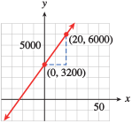
Find an equation for the line shown in FigureΒ 1.136.
described in detail following the image
graph of line
Figure 1.136.
Solution.
The line crosses the \(y\)-axis at the point \((0, 3200)\text{,}\) so \(b=3200\text{.}\) To calculate the slope of the line, we locate another point, say \((20, 6000)\text{,}\) and compute:
\begin{align*} m \amp = \frac{\Delta y}{\Delta x} = \frac{6000 - 3200}{20 - 0}\\ \amp =\frac{2800}{20}= 140 \end{align*}
The slope-intercept form of the equation, with \(m = 140\) and \(b = 3200\text{,}\) is
\begin{equation*} y = 3200 + 140x\text{.} \end{equation*}
described in detail following the image
graph of line
Figure 1.137.

Example 1.138.

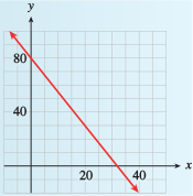
Find an equation for the line shown in FigureΒ 1.139.
described in detail following the image
graph of line
Figure 1.139.
Solution.
The line crosses the \(y\)-axis at the point \((0, 80)\text{,}\) so \(b=80\text{.}\) To calculate the slope of the line, we locate another point, say \((20,30)\text{,}\) and compute:
\begin{equation*} \begin{aligned}m \amp = \frac{\Delta y}{\Delta x} = \frac{30 - 80}{20 - 0}\\ \amp =\frac{-50}{20}= -\frac{5}{2} \end{aligned} \end{equation*}
The slope-intercept form of the equation is
\begin{equation*} y = 80 - \frac{5}{2}x\text{.} \end{equation*}

Subsection 1.6.2 Point-Slope Form

We can find an equation for a line if we know its slope and \(y\)-intercept. What if we do not know the \(y\)-intercept, but instead know some other point on the line? There is only one line that passes through a given point and has a given slope, so we should be able to find an equation for this line.
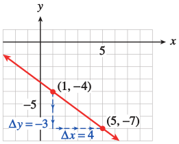
For example, we can graph the line of slope \(\dfrac{-3}{4}\) that passes through the point \((1, -4)\text{.}\) We first plot the given point, \((1, -4)\text{,}\) as shown in FigureΒ 1.140.
Then we use the slope to find another point on the line. The slope is
\begin{equation*} m =\frac{-3}{4}= \frac{\Delta y}{\Delta x} \end{equation*}
so we move down \(3\) units and then \(4\) units to the right, starting from \((1, -4)\text{.}\) This brings us to the point \((5, -7)\text{.}\) We can then draw the line through these two points.
described in detail following the image
point slope
Figure 1.140.
We can also find an equation for the line, as shown in ExampleΒ 1.141.

Example 1.141.

Find an equation for the line that passes through \((1, -4)\) and has slope \(\dfrac{-3}{4}\text{.}\)
Solution.
We will use the formula for slope,
\begin{equation*} m = \frac{y_2 - y_1}{x_2 - x_1}. \end{equation*}
We substitute \(\dfrac{-3}{4}\) for the slope, \(m\text{,}\) and \((1, -4)\) for \((x_1, y_1)\text{.}\) For the second point, \((x_2, y_2)\text{,}\) we use the variable point \((x, y)\text{.}\) Substituting these values into the slope formula gives us
\begin{equation*} \frac{-3}{4}= \frac{y - (-4)}{x - 1}=\frac{y + 4}{x - 1}. \end{equation*}
To solve for \(y\) we first multiply both sides by \(x - 1\text{.}\)
\begin{align*} \alert{(x-1)}\frac{-3}{4}\amp =\frac{y +4}{x - 1}\alert{(x-1)} \amp\amp\\ \frac{-3}{4}(x-1)\amp=y+4 \amp\amp\text{Apply the distributive law.}\\ \frac{-3}{4}x+\frac{3}{4}\amp=y+4 \amp\amp \text{Subtract 4 from both sides.}\\ \frac{-3}{4}x-\frac{13}{4}\amp=y \amp\amp \frac{3}{4}-4=\frac{3}{4}-\frac{16}{4}=\frac{-13}{4} \end{align*}
An equation of the line is \(y=\dfrac{-13}{4}-\dfrac{3}{4}x.\)

When we use the slope formula in this way to find an equation of a line, we substitute a variable point \((x, y)\) for the second point. This version of the formula,
\begin{equation*} m = \frac{y - y_1}{x - x_1} \end{equation*}
is called the point-slope form for a linear equation. It is sometimes stated in another form obtained by clearing the fraction to get
\begin{align*} \alert{(x-x_1)}m\amp =\frac{y -y_1}{x - x_1}\alert{(x-x_1)} \amp\amp \text{Multiply both sides by }(x - x_1)\\ (x - x_1) m\amp=y-y_1 \amp\amp\text{Clear fractions and solve for }y\text{.}\\ y\amp=y_1+m(x-x_1). \end{align*}

Point-Slope Form.

An equation of the line that passes through the point \((x_1, y_1)\) and has slope \(m\) is
\begin{equation*} y= y_1 + m(x- x_1). \end{equation*}

Example 1.142.

Use the point-slope form to find an equation of the line that passes through the point \((-3, 5)\) and has slope \(-1.4\text{.}\)
Solution.
Subsituting \(m=-1.4\) and \((-3,5)\) for \((x_1,y_1)\) into the point-slope form of a line, we have
\begin{equation*} \begin{aligned} y\amp=5-1.4(x-(-3)) \\ y\amp=0.8-1.4x \end{aligned} \end{equation*}
The point-slope form is useful for modeling linear functions when we do not know the initial value but do know some other point on the line.

Example 1.143.

Under a proposed graduated income tax system, single taxpayers would owe $1500 plus 20% of the amount of their income over $13,000. (For example, if your income is $18,000, you would pay $1500 plus 20% of $5000.)
  1. Complete the table of values for the tax, \(T\text{,}\) on various incomes, \(I\text{.}\)
    \(I\) \(15,000\) \(20,000\) \(22,000\)
    \(T\)
  2. Write a linear equation in point-slope form for the tax, \(T\text{,}\) on an income \(I\text{.}\)
  3. Write the equation in slope-intercept form.
Solution.
  1. On an income of $15,000, the amount of income over $13,000 is $15,000 - $13,000 = $2000, so you would pay $1500 plus 20% of $2000, or
    \begin{equation*} T = 1500 + 0.20(2000) = 1900. \end{equation*}
    You can compute the other function values in the same way.
    \(I\) \(15,000\) \(20,000\) \(22,000\)
    \(T\) \(1900\) \(2900\) \(3300\)
  2. On an income of \(I\text{,}\) the amount of income over $13,000 is \(I - \$13,000\text{,}\) so you would pay $1500 plus 20% of \(I - 13,000\text{,}\) or
    \begin{equation*} T = 1500 + 0.20 (I - 13,000). \end{equation*}
  3. Simplify the right side of the equation to get
    \begin{align*} T \amp = 1500 + 0.20I - 2600\\ T \amp = -1100 + 0.20I. \end{align*}

Example 1.144.

A healthy weight for a young woman of average height, 64 inches, is 120 pounds. To calculate a healthy weight for a woman taller than 64 inches, add 5 pounds for each inch of height over 64.
  1. Write a linear equation in point-slope form for the healthy weight, \(W\text{,}\) for a woman of height, \(H\text{,}\) in inches.
  2. Write the equation in slope-intercept form.
Solution.
  1. \(\displaystyle W = 120 + 5(H - 64)\)
  2. \(\displaystyle W = -200 + 5H\)
If you would like more information on linear equations, refer to the following two sections from Intermediate Algebra:

Exercises 1.6.3 Exercises

1. Using a Table to Find a Linear Function.

Determine whether the following table could represent a linear function. If it can, find a possible formula for the linear function in \(y=mx+b\) form. If it can’t, please write "NONE" in the formula line.
\(x\) \(-5\) \(-3\) \(0\) \(5\)
\(g(x)\) \(-38\) \(-20\) \(7\) \(52\)
Formula: \(f(x)=\)
\(x\) \(-5\) \(-3\) \(0\) \(5\)
\(f(x)\) \(41\) \(31\) \(6\) \(-26\)
Formula: \(g(x)=\)
Hint.
In order for a function to be linear, it needs to have a constant average rate of change. Therefore, to determine if these tables represent linear functions, we need to calculate the average rate of change over each interval on the table. Recall the average rate of change formula on an interval \([a,b]\text{:}\)
\begin{equation*} \frac{f(b)-f(a)}{b-a}. \end{equation*}
a) Find the average rate of change on the intervals \([-5,-3]\text{,}\) \([-3,0]\text{,}\) \([0,5]\text{.}\)
If each average rate of change is the same, this is a linear function. You can use slope-intercept form \((y=mx+b)\) or point-slope form \((y=y_1+m(x-x_1))\) to find the equation.
b) The process will be the same for the second table.

2. Finding a Linear Function from Points.

Find a formula for a line that
a) has slope \(3\) and passes through the point \((-1,-4)\text{.}\)
\(y=\)
b) passes through the points \((-1,3)\) and \((5,-3)\text{.}\)
\(y=\)
Hint.
a) We are given the slope of 3 and the point \((-1,-4)\text{.}\) We can use Point-Slope Form to write an equation for the line:
\begin{equation*} y=y_1+m(x-x_1). \end{equation*}
b) We need to find the slope of the line using the given points in this case. Recall the formula for slope:
\begin{equation*} m=\frac{y_2-y_1}{x_2-x_1}. \end{equation*}
Then we can use Point-Slope Form to write an equation for the line using either of the given points.
NOTE: You could also write these equations in Slope-Intercept Form by finding the vertical intercept.

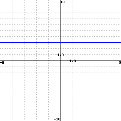
3. Finding a Linear Function from a Graph.

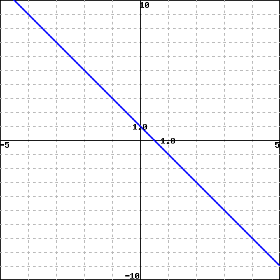
Find a formula for each of the following lines. Use any form you wish.
\(y=\)
\(y=\)
Hint.
a) We need to find the slope of the line using the graph in this case. Recall the formula for slope is
\begin{equation*} m=\frac{y_2-y_1}{x_2-x_1}. \end{equation*}
We can see that the vertical intercept is given by the point \((0,1)\text{.}\)
Then we can use Slope-Intercept Form to write an equation for the line:
\begin{equation*} y=m x+b. \end{equation*}
b) In this case, we have a horizontal line. You can think about the slope of this line and find the vertical intercept to put into the equation given above.

4. Applications of Linear Functions.

The population of a town in 1920 was 2700 people. The town’s population decreased linearly, and in 1923 the population was 2580. Find a formula for \(P\text{,}\) the town’s population, in terms of \(t\text{,}\) the number of years since 1920.
\(P(t) = \ \)

5. Applications of Linear Functions.

You bought a new car for $19,500 in 2005, and the value of the car depreciates by $500 each year. Find a formula for \(V\text{,}\) the value of the car in dollars, in terms of \(t\text{,}\) the number of years since 2005.
\(V(t) = \ \)
(Be sure NOT TO USE ANY COMMAS when you enter your formula. For example enter two thousand as 2000 and not as 2,000.)

6. Finding Linear Functions Given Properties.

Find an equation for the linear function whose graph has its \(y\)-intercept at \(y=\)-2 and \(x\)-intercept at \(x=\)11.
\(f(x) =\)