
Supplemental Videos
The main topics of this section are also presented in the following videos:
The main topics of this section are also presented in the following videos:
We have already encountered some examples of polynomial functions. Linear functions,
and quadratic functions
are special cases of polynomial functions. In general, we make the following definition.
A polynomial function is a function which can be written in the form
where \(a_0\text{,}\) \(a_1\text{,}\) \(a_2\text{,}\) \(\ldots\text{,}\) \(a_n\) are constants and \(a_n \ne 0\text{.}\)
The parts making up the polynomial function which are of the form \(a_ix^i \) for some \(i \) are called terms. The term \(a_nx^n \) is call the leading term.
The coefficient \(a_n\) of the highest power term is called the leading coefficient.
The power of \(x \) appearing in the leading term (in this case \(n \)), is the degree of the polynomial.
Some examples of polynomials are
Each of the polynomials above is written in descending powers, which means that the highest-degree term comes first, and the degrees of the terms decrease from largest to smallest. Sometimes it is useful to write a polynomial in ascending powers, so that the degrees of the terms increase. For example, the polynomial \(f(x)\) above would be written as
in ascending powers.
Note that \(f(x)\) has four non-zero terms, namely
Since the term of \(f(x) \) of highest degree is \(6x^{\alert{3}}\text{,}\) we say that \(f(x)\) has degree \(\alert{3}\text{.}\)
Let's just jump right into an example!
Compute the products.
Multiply \((y + 2)(y^2 - 2y + 3)\text{.}\)
In Example320a, we multiplied a polynomial of degree 1 by a polynomial of degree 3, and the product was a polynomial of degree 4. In Example320b, the product of three first degree polynomials is a third-degree polynomial. In Example321, we multiplied a polynomial of degree 1 by a polynomial of degree 2, and the product was a polynomial is of degree 3. You might notice that the degree of the product is always the sum of the degrees of the factors; this is a useful property of polynomials that allows us to find the degree of a product without computing it.
The degree of a product of nonzero polynomials is the sum of the degrees of the factors. That is,
if \(P(x)\) has degree \(m\) and \(Q(x)\) has degree \(n\) (and both \(P(x)\) and \(Q(x)\) are nonzero), then their product \(P(x)Q(x)\) has degree \(n + m\text{.}\)
Let \(P(x) = 5x^4 - 2x^3 + 6x^2 - x + 2\text{,}\) and \(Q(x) = 3x^3 - 4x^2 + 5x + 3\text{.}\)
What is the degree of their product? What is the coefficient of the lead term?
Find the coefficient of the \(x^3\)-term of the product.
The degree of \(P\) is \(4\text{,}\) and the degree of \(Q\) is \(3\text{,}\) so the degree of their product is \(4 + 3 = 7\text{.}\) The only degree \(7\) term of the product is \((5x^4)(3x^3) = 15x^7\text{,}\) which has coefficient \(15\text{.}\)
In the product, each term of \(P(x)\) is multiplied by each term of \(Q(x)\text{.}\) We get degree \(3\) terms by multiplying together terms of degree \(0\) and \(3\text{,}\) or \(1\) and \(2\text{.}\) For these polynomials, the possible combinations are:
| \(P(x)\) | \(Q(x)\) | Product |
| \(2\) | \(3x^3\) | \(6x^3\) |
| \(-2x^3\) | \(3\) | \(-6x^3\) |
| \(-x\) | \(-4x^2\) | \(4x^3\) |
| \(6x^2\) | \(5x\) | \(30x^3\) |
The sum of the third-degree terms of the product is \(34x^3\text{,}\) with coefficient \(34\text{.}\)
Let \(f(x) = 2x^6 + 2x^4 - x^3 + 5x^2 + 1\) and \(g(x) = x^5 - 3x^4 + 2x^3 + x^2 - 4x - 2\text{.}\)
What is the degree of their product? What is the coefficient of the lead term?
Find the coefficient of the \(x^4\)-term of the product.
The degree of \(f\) is \(6\text{,}\) and the degree of \(g\) is \(5\text{,}\) so the degree of their product is \(6 + 5 = 11\text{.}\) The only degree \(11\) term of the product is \((2x^6)(x^5) = 2x^{11}\text{,}\) which has coefficient \(2\text{.}\)
In the product, each term of \(f(x)\) is multiplied by each term of \(g(x)\text{.}\) We get degree \(4\) terms by multiplying together terms of degree \(0\) and \(4\text{,}\) \(1\) and \(3\text{,}\) or \(2\) and \(2\text{.}\) For these polynomials, the possible combinations are:
| \(f(x)\) | \(g(x)\) | Product |
| \(2x^4\) | \(-2\) | \(-4x^4\) |
| \(-x^3\) | \(-4x\) | \(4x^4\) |
| \(5x^2\) | \(x^2\) | \(5x^4\) |
| \(1\) | \(-3x^4\) | \(-3x^4\) |
The sum of the fourth-degree terms of the product is \(2x^4\text{,}\) with coefficient \(2\text{.}\)
The graph of a polynomial function depends first of all on its degree. We have already studied the graphs of polynomials of degrees \(0\text{,}\) \(1\text{,}\) and \(2\text{.}\)

Quadratic functions, such as \(f(x) = -2x^2 + 6x + 8\text{,}\) are polynomials of degree \(2\text{.}\) The graph of every quadratic function is a parabola, with the same basic shape as the standard parabola, \(y = x^2\text{.}\) (See Figure325.) Notice that the graph changes from increasing to decreasing or vice versa at one point. This point of a parabola is the same as its vertex (which we defined in section 10.2).

Do the graphs of all cubic, or third-degree, polynomials have a basic shape in common? We can graph a few examples and find out. Unlike the basic parabola, the graph of \(y = x^3\) is always increasing. At the origin, however, it changes from concave down to concave up. A point where the graph changes concavity is called an inflection point. You do not need to concern yourself with concavity and inflection points in this course. However, if you continue on to Calculus, this definition will appear again!
Graph the cubic polynomial \(P(x) = x^3 - 4x\) and compare its graph with that of the basic cubic, \(y = x^3\text{.}\)
The graph of the basic cubic is shown in Figure327a. To help us understand the graph of the polynomial \(P(x) = x^3 - 4x\text{,}\) we will evaluate the function to make a table of values. We can do this by hand or use the Table feature on the graphing calculator.

| \(x\) | \(-3\) | \(-2\) | \(-1\) | \(0\) | \(1\) | \(2\) | \(3\) |
| \(P(x)\) | \(-15\) | \(0\) | \(3\) | \(0\) | \(-3\) | \(0\) | \(15\) |
The graph of \(P(x) = x^3 - 4x\) is shown in Figure327b. While the graph of \(P(x)\) does not look exactly like the graph of \(y=x^3\text{,}\) it is similar, especially at the edges of the graphs.
Despite the differences in the central portions of the two graphs, they exhibit similar long-run behavior.
All cubic polynomials display this behavior when their lead coefficients (the coefficient of the \(x^3\) term) are positive.
Complete the table of values below for \(C(x) = -x^3 - 2x^2 + 4x + 4\text{.}\)
| \(x\) | \(-4\) | \(-3\) | \(-2\) | \(-1\) | \(0\) | \(1\) | \(2\) | \(3\) | \(4\) |
| \(y\) | \(\hphantom{000}\) | \(\hphantom{000}\) | \(\hphantom{000}\) | \(\hphantom{000}\) | \(\hphantom{000}\) | \(\hphantom{000}\) | \(\hphantom{000}\) | \(\hphantom{000}\) | \(\hphantom{000}\) |
Graph \(y = C(x)\) in the standard window. Compare the graph to the graphs in Example326: What similarities do you notice? What differences?
| \(x\) | \(-4\) | \(-3\) | \(-2\) | \(-1\) | \(0\) | \(1\) | \(2\) | \(3\) | \(4\) |
| \(y\) | \(20\) | \(1\) | \(-4\) | \(-1\) | \(4\) | \(5\) | \(-4\) | \(-29\) | \(-76\) |
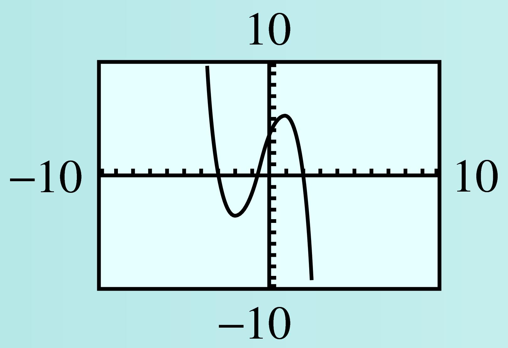
Both graphs have three \(x\)-intercepts, but the function in Example326 has long-term behavior like \(y = x^3\text{,}\) and this function has long-term behavior like \(y = -x^3\text{.}\)
Now let's compare the long-term behavior of two quartic, or fourth-degree, polynomials.
Graph the polynomials \(f(x) = x^4 - 10x^2 + 9\) and \(g(x) = x^4 + 2x^3\text{,}\) and compare.
For each function we make a table of values.
| \(x\) | \(-4\) | \(-3\) | \(-2\) | \(-1\) | \(0\) | \(1\) | \(2\) | \(3\) | \(4\) |
| \(f(x)\) | \(105\) | \(0\) | \(-15\) | \(0\) | \(9\) | \(0\) | \(-15\) | \(0\) | \(105\) |
| \(G(x)\) | \(128\) | \(27\) | \(0\) | \(-1\) | \(0\) | \(3\) | \(32\) | \(135\) | \(384\) |
The graphs are shown in Figure330. All the essential features of the graphs are shown in these viewing windows. The graphs continue forever in the directions indicated, without any additional twists or turns. You can see that the graph of \(f\) has three turning points, and the graph of \(g\) has one turning point.

As in Example326, both graphs have similar long-term behavior. The \(y\)-values decrease from \(-\infty\) toward zero as \(x\) increases from \(-\infty\text{,}\) and the \(y\)-values increase toward \(+\infty\) as \(x\) increases to \(+\infty\text{.}\) This long-term behavior is similar to that of the power function \(y = x^4\text{.}\) Its graph also starts at the upper left and extends to the upper right.
Complete the following table of values for \(Q(x) = -x^4 - x^3 - 6x^2 + 2\text{.}\)
| \(x\) | \(-4\) | \(-3\) | \(-2\) | \(-1\) | \(0\) | \(1\) | \(2\) | \(3\) | \(4\) |
| \(y\) | \(\hphantom{000}\) | \(\hphantom{000}\) | \(\hphantom{000}\) | \(\hphantom{000}\) | \(\hphantom{000}\) | \(\hphantom{000}\) | \(\hphantom{000}\) | \(\hphantom{000}\) | \(\hphantom{000}\) |
Graph \(y = Q(x)\) in the window \begin{align} \text{Xmin} \amp = -5 \amp\amp \text{Xmax} = 5\\ \text{Ymin} \amp = -15 \amp\amp \text{Ymax} = 10. \end{align} Compare the graph to the graphs in Example329: What similarities do you notice? What differences?
| \(x\) | \(-4\) | \(-3\) | \(-2\) | \(-1\) | \(0\) | \(1\) | \(2\) | \(3\) | \(4\) |
| \(y\) | \(-286\) | \(-106\) | \(-30\) | \(-4\) | \(2\) | \(-6\) | \(-48\) | \(-160\) | \(-414\) |
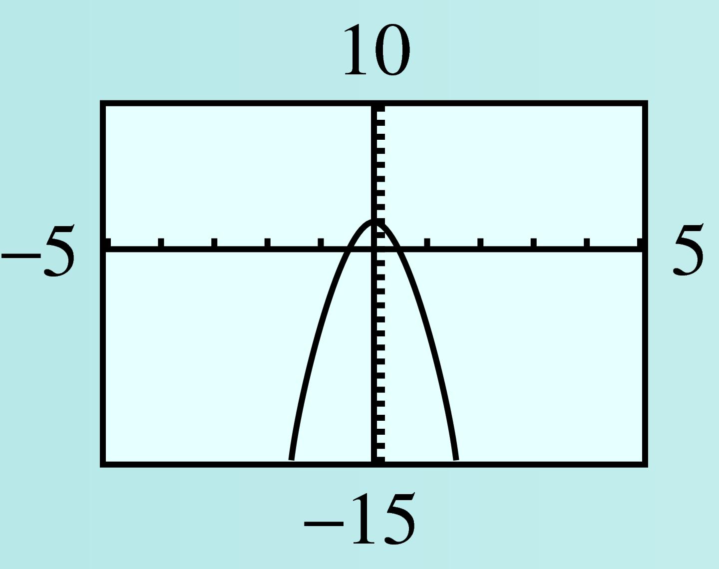
The graphs all have long-term behavior like a fourth degree power function, \(y = ax^4\text{.}\) The long-term behavior of the graphs in Example329 is the same as that of \(y = x^4\text{,}\) but the graph here has long-term behavior like \(y = -x^4\text{.}\)
In the exercises, you will consider more graphs to help you verify the following observations.
A polynomial of odd degree (with positive leading coefficient) has negative \(y\)-values for large negative \(x\)-values and positive \(y\)-values for large positive \(x\)-values. In general, this type of polynomial will have a graph similar to graph (a) below.
A polynomial of even degree (with positive leading coefficient) has positive \(y\)-values for both large positive and large negative \(x\)-values. In general, this type of polynomial will have a graph similar to graph (b) below.

