Josh Brummer, Taran Funk, Lawrence Seminario-Romero, Ariel Setniker, Karina Uhing, Nathan Wakefield, Catherine Zimmitti, The Mabel Elizabeth Kelly Fund
Last section, we categorized polynomials by the long-run behavior. We now take a closer look at how these functions behave for smaller \(x\)-values. In particular, we see how the polynomial behaves around its roots.
In this section, we will pay close attention to the factors of polynomials. Just like we factored quadratic functions, we can factor polynomials of higher degrees. A polynomial is in factored form if it looks like \(f(x)=f_1(x) \cdot f_2(x) \cdot \ldots \cdot f_k(x)\) and each of the factors \(f_1(x), f_2(x), \ldots, f_3(x)\) cannot be factored further.
Subsection8.2.1\(x\)-Intercepts (roots) and Short-Run Behavior
We have seen before that the \(x\)-intercepts of a quadratic polynomial, \(f(x) = ax^2 + bx + c\text{,}\) occur at values of \(x\) for which \(f(x) = 0\text{,}\) that is, at the real-valued solutions of the equation \(ax^2 + bx + c = 0\text{.}\) The same holds true for polynomials of higher degree.
Solutions of the equation \(P(x) = 0\) are called zeros of the polynomial \(P\text{.}\) In Example 8.7, we graphed the cubic polynomial \(P(x) = x^3 - 4x\text{.}\) Its \(x\)-intercepts are the solutions of the equation \(x^3 - 4x = 0\text{,}\) which we can solve by factoring the polynomial \(P(x)\text{.}\)
The zeros of \(P\) are \(0\text{,}\)\(2\text{,}\) and \(-2\text{.}\) Each zero of \(P\) corresponds to a linear factor of \(P(x)\text{.}\) This result suggests the following theorem, which holds for any polynomial \(P\text{.}\)
Because a polynomial function of degree \(n\) can have at most \(n\) linear factors of the form \((x - a)\text{,}\) it follows that \(P\) can have at most \(n\) distinct zeros. If a zero appears more than once, we describe the number of times it appears as the multiplicity.
Another way of saying this is that if \(P(x)\) is a polynomial of degree \(n\text{,}\) the equation \(P(x) = 0\) can have at most \(n\) distinct solutions.
Not every function will factor into linear factors. If the there are non-linear factors after the function is fully factored, some solutions will be complex numbers. For example, the function \(x^3 + x = x(x^2 + 1)\) has one linear factor, \(x \text{,}\) and one non-linear factor, \(x^2 + 1 \text{,}\) which can’t be factored further, so the only real solution is \(x = 0\) (the other two solutions are complex numbers). We do not cover complex numbers in this course but there are plenty of reasonable resources available online if you wish to know more.
If some of the zeros of \(P\) are complex numbers, they will not appear on the graph, so a polynomial of degree \(n\)may have fewer than \(n\)\(x\)-intercepts.
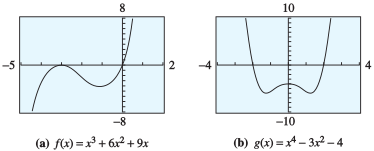
By the factor theorem, the zeros of \(f\) are \(0\text{,}\)\(-3\text{,}\) and \(-3\text{.}\) (We say that \(f\) has a zero of multiplicity two at \(-3\text{.}\)) Because all of these are real numbers, all will appear as \(x\)-intercepts on the graph. Thus, the \(x\)-intercepts occur at \((0, 0)\) and at \((-3, 0)\text{.}\)
Because \(x^2 + 1\) cannot be factored in real numbers, the graph has only two \(x\)-intercepts, at \((-2, 0)\) and \((2, 0)\text{.}\) Hence, \(g(x)\) has only \(x=-2\) and \(x=2\) as its zeros. The graphs of both polynomials are shown in Figure 8.15.
The appearance of the graph near an \(x\)-intercept is determined by the multiplicity of the zero there. For example, both real zeros of the polynomial \(g(x) = x^4 - 3x^2 - 4\) in Example 8.14b are of multiplicity one, and the graph crosses the \(x\)-axis at each intercept.
However, the polynomial \(f(x) = x^3 + 6x^2 + 9x\) in Example 8.14a has a zero of multiplicity two at \(x = -3\text{.}\) The graph of \(f\) just touches the \(x\)-axis and then reverses direction without crossing the axis.
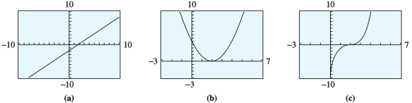
In Figure 8.17b, \(Q(x) = (x - 2)^2\) has a zero of multiplicity two at \(x = 2\text{,}\) and its graph touches the \(x\)-axis there but changes direction without crossing.
In Figure 8.17c, \(C(x) = (x - 2)^3\) has a zero of multiplicity three at \(x = 2\text{.}\) In this case, the graph makes an S-shaped curve at the intercept, like the graph of \(y = x^3\text{.}\)
Although we will not consider zeros of multiplicity greater than three, they correspond to similar behavior in the graph: At a zero of odd multiplicity, the graph has an inflection point at the intercept; its graph makes an S-shaped curve. At a zero of even multiplicity, the graph has a turning point; it changes direction without crossing the \(x\)-axis.
The polynomial has degree six, an even number, so its graph starts at the upper left and extends to the upper right. The \(y\)-coordinate of the \(y\)-intercept is
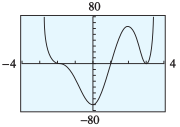
Note that \(f\) has a zero of multiplicity three at \(x = -2\text{,}\) a zero of multiplicity one at \(x = 1\text{,}\) and a zero of multiplicity two at \(x = 3\text{.}\) The graph has an S-shaped curve at \(x = -2\text{,}\) crosses the \(x\)-axis at \(x = 1\text{,}\) touches the \(x\)-axis at \(x = 3\text{,}\) and then changes direction, as shown in Figure 8.20.
a) Recall the zeros are where the function’s graph crosses the horizontal axis. In other words, where the output is 0. So we can find this information by setting the function equal to 0. It may be useful to factor the function completely to answer this question.
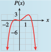
For the long-run behavior of this function, consider the long-run behavior of the leading term. In this case, the polynomial is a downward facing parabola. Think about what that means as \(x\) goes to \(\infty\) and \(-\infty\text{.}\)
Using an online tool, determine the number of zeros (i.e., the number of times the function makes contact with the \(x\)-axis) of the polynomial \(f(x)=x^5 + 2.8 x^4 + 5.96 x^3 + 11.2 x^2 + 7.84 x\text{.}\) Again using this online tool, estimate these zeros. Is the multiplicity of each zero even or odd?
A zero with even multiplicity will look like it bounces off the \(x\)-axis on the graph. A zero with odd multiplicity will cross the \(x\)-axis on the graph.
Complete the following table using the formulas for each of the above functions and any additional information you can obtain from the graph of each function. You may want to sketch graphs on your own piece of paper. You are welcome to use an online graphing utility like www.desmos.com if you would like
b) In the order the roots appear in the factored forms of the functions provided, list the roots, the multiplicity of the roots, and if the function "bounces" off or "crosses" the \(x\)-axis at that root. If there are more blanks provided than needed for a given function, enter NONE in all remaining, unneeded blanks. Most of the information for function \(f(x)\) has been completed as an example.
Recall the leading term is the term in the polynomial with the largest valued exponent. The degree of a polynomial is the value of the largest exponent (it’s the exponent on the leading term).
The multiplicity of a zero is given by the exponent of the factor. For example, the zero \(x=0\) has multiplicity 2 in \(f(x)\) above. From looking at the graph of the function, you can determine if the function bounces off the \(x\)-axis or crosses the \(x\)-axis at each given zero.
a) Let \(k(x) = 2 (x + 5)(x^2-16)\text{.}\) What are the zeros of \(k\text{?}\) The \(y\)-intercept? Enter the zeros in order from smallest to largest. If there are more blanks provided than you need for the zeros, enter "NONE" for the remaining ordered pairs.
a) To find all zeros, it may be useful to factor the function completely. Recall the zeros occur when the output is 0, so you can set the equation equal to 0.
b) Recall the long-run behavior of a polynomial is the same as the long-run behavior of its leading term. Find the leading term of the polynomial to determine the long-run behavior.
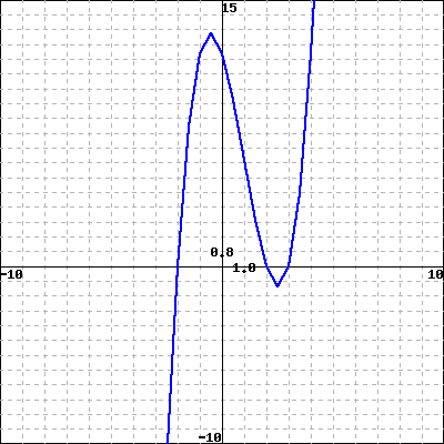
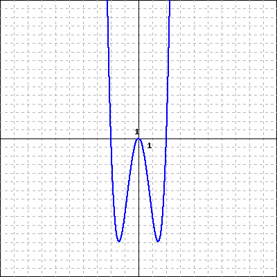
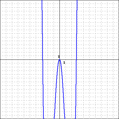
Find the zeros on the graph and determine if they should have even or odd multiplicity (recall odd multiplicity means the function will cross the \(x\)-axis at the \(x\)-intercept and even multiplicity means the function will bounce off the \(x\)-axis at the \(x\)-intercept). We want the least degree polynomial, so you should choose multiplicity 1 (for odd multiplicities) or 2 (for even multiplicities).
Select a possible formula for the polynomial \(f(x)\text{,}\) given that \(f(x)\) has degree three, \(f(-2)=f(2)=f(6)=0\text{,}\) and \(\lim_{x\to \infty}f(x)=-\infty\text{.}\)
Determine what \(f(-2)=0\) means in this context/what information that gives you. Try to write an equation in factored form for the function \(f(x)\text{.}\)
Try to find the \(x\)-intercepts of the given function and the long-run behavior. It may be useful to factor the function completely to see what the multiplicities are (to determine if the function should bounce or cross at a given \(x\)-intercept).
a) Letting \(x\) denote the length of one of the sides of the bottom of the box, and letting \(y\) denote the height of the box, sketch a picture of the box, labeling the length, width, and height. The company wants to use exactly 121 cm\(^{2}\) of material for the box. That is, the box’s surface area will be equal to 121 cm\(^{2}\text{.}\) Write an equation in terms of \(x\) and \(y\) representing this constraint, putting the variables on the left side.
b) Using your work from part (a), write a formula for the volume of the box, \(V(x)\text{,}\) as a function of \(x\text{.}\) Simplify as much as possible.
c) Use an online source to approximate the maximum value of \(V(x)\) on the interval \([0,10]\text{.}\) What \(x\) value corresponds to this maximum value?
a) To find the surface area of a box, we want to add up the area of each side. Use the given information to find the area of each side of the box and add them all together. This expression should be set equal to the given surface area.
b) Try to write an equation for the volume of the box, using \(x\) and \(y). Once you have that equation, plug in the equation from part a) for \(y\text{.}\)
c) Graph the equation from part b) (we recommend using Desmos). Use the graph to find the appropriate value of \(x\) in the given domain. Think about what the units are for the value of \(x\) to give the right interpretation.