Josh Brummer, Taran Funk, Lawrence Seminario-Romero, Ariel Setniker, Karina Uhing, Nathan Wakefield, Catherine Zimmitti, The Mabel Elizabeth Kelly Fund
In the previous section we listed some properties of exponential functions without much justification. In this section we will discuss why these properties hold, and investigate the long-run behavior of exponential functions.
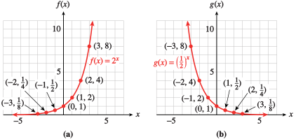
The graphs of exponential functions have two characteristic shapes, depending on whether the base, \(b\text{,}\) is greater than \(1\) or less than \(1\text{.}\) As typical examples, consider the graphs of \(f (x) = 2^x\) and \(g(x) =\left(\dfrac{1}{2}\right)^x\) shown in Figure 3.17. Some values for \(f\) and \(g\) are recorded in Tables 3.15 and 3.16.
Notice that \(f (x) = 2^x\) is an increasing function and \(g(x) = \left(\dfrac{1}{2}\right)^x\) is a decreasing function. In general, exponential functions have the following properties.
In Table 3.15 you can see that as the \(x\)-values decrease toward negative infinity, the corresponding \(y\)-values decrease toward zero. As a result, the graph of \(f\) decreases toward the \(x\)-axis as we move to the left. Thus, the \(x\)-axis, \(y=0 \text{,}\) is a horizontal asymptote for exponential functions no matter what value \(b\text{,}\) the growth factor, happens to be. We can see this illustrated in Figure 3.17, since the \(y\)-values of each exponential get closer to zero. (For more info on horizontal asymptotes, see Appendix B.)
For exponential functions with \(0 \lt b \lt 1\text{,}\) this takes place close to the positive \(x\)-axis, as illustrated in Figure 3.17b. For exponential functions with \(1 \lt b\text{,}\) this takes place close to the negative \(x\)-axis, as illustrated in Figure 3.17a.
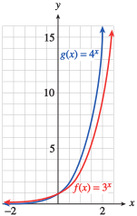
In Example 3.18, we compare two increasing exponential functions. The larger the value of the base, \(b\text{,}\) the faster the function grows. In this example, both functions have \(a = 1\text{.}\)
Plot the points for each function and connect them with smooth curves. For positive \(x\)-values, \(g(x)\) is always larger than \(f (x)\text{,}\) and is increasing more rapidly. In Figure 3.20, \(g(x) = 4^x\) climbs more rapidly than \(f (x) = 3^x\text{.}\) Both graphs cross the \(y\)-axis at (0, 1).
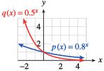
For decreasing exponential functions, those with bases between \(0\) and \(1\text{,}\) the smaller the base, the more steeply the graph decreases. For example, compare the graphs of \(p(x) = 0.8^x\) and \(q(x) = 0.5^x\) shown in Figure 3.21.
On the domain \([-2,2]\text{,}\) the smallest values for both \(f\) and \(g\) occur when \(x=-2\text{,}\) and the largest values occur when \(x=2\) (since both of these functions are increasing). Since
the range of \(f\) on the domain \([-2,2]\) is \(\left[\frac{1}{9},9\right]\text{;}\) the range of \(g\) on the domain \([-2,2]\) is \(\left[\frac{1}{16},16\right]\text{.}\)
On the domain \([-2,2]\text{,}\) the smallest values for both \(p\) and \(q\) occurs when \(x=2\text{,}\) and the largest values occurs when \(x=-2\) (since both of these functions are decreasing). Since
the range of \(p\) on the domain \([-2,2]\) is \(\left[0.25,4\right]\text{;}\) the range of \(q\) on the domain \([-2,2]\) is \(\left[0.64,1.5625\right]\text{.}\)
Suppose a certain population of bacteria is known to grow by 16 percent each day. If a lab has 1200 bacteria on May 1, how many bacteria will there be 25 days from then?
Use this information to write an equation that gives the population of bacteria as a function of \(t\) days. Then you’ll want to evaluate this equation.
where \(a\) is the initial value and \(b\) is the growth factor. We know \(b=1+r\text{,}\) where \(r\) is the growth rate. Note here that the number of cases is decreasing, so \(r\) should be negative.
The Emerald City’s population density shrunk throughout the 1970s. In 1970, the population density was approximately 7710 people per square mile, and it was shrinking at a rate of 0.8 percent per year.
where \(a\) is the initial value and \(b\) is the growth factor. We know \(b=1+r\text{,}\) where \(r\) is the growth rate. Note here that the population density is decreasing, so \(r\) should be negative.
Suppose that the percentage of children not vaccinated against the disease Dermatitis is given by the equation \(V(t)=3+97(0.84)^t\text{,}\) where \(t\) is in years since 1950. As \(t\) goes to infinity, what happens to \(V(t)\text{?}\) What does this mean in practical terms? Select the answer that best fits the situation.
Try to plug in a very large positive number for \(t\) to symbolize \(t\) going to infinity. You may want to plug in increasing numbers to see what values the function \(V(t)\) is getting closer and closer to.
b) Graph both \(f(x)\) and \(g(x)\) on your own piece of paper, then compute the average rate of change for both functions on the intervals \([0,5]\) and \([5,10]\text{.}\)
b) The formula for the average rate of change over an interval for \(f(x)\) is given by \(\frac{f(b) - f(a)}{b-a}\text{,}\) where \(a\) is the left endpoint of the interval and \(b\) is the right endpoint of the interval. Calculate the average rate of change on each interval using this information and the given functions.
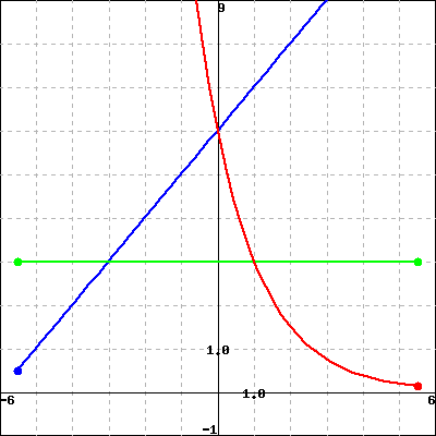
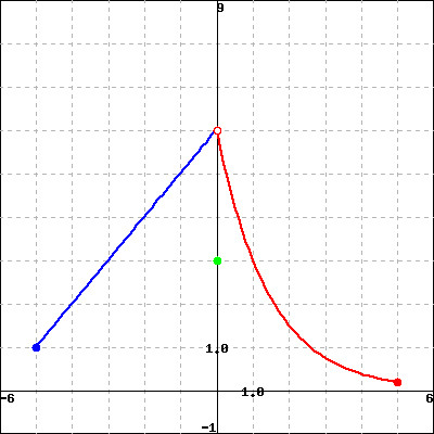
Use the function \(g(x)\) as defined below to answer parts (a)-(d). \(\begin{align*}
g(x) =
\begin{cases}
x+6, \amp x\lt 0\\
3, \amp x=0\\
6(0.5)^x, \amp x>0
\end{cases}
\end{align*}\)
b) Use the graph from part a) to help you figure this out. Recall the domain is the set (interval) of all possible input values and the range is the set (interval) of associated output values.
c) Use the graph from part a) to help you figure this out. Recall a function is increasing if it looks like it’s "going up" as you move from left to right and a function is decreasing if it looks like it’s "going down" as you move from left to right.
d) Think about what happens to the values of the function as you plug in larger and larger values of \(x\text{.}\) In other words, what value is the function getting closer to as you move to the right on the input axis?
If the function is approaching a constant number (not infinity), the function has a horizontal asymptote. Horizontal asymptotes are lines of the form \(y=k\) for some constant \(k\text{.}\)