Section 8.1 Polynomial Functions

Supplemental Videos.

The main topics of this section are also presented in the following videos:

We have already encountered some examples of polynomial functions. Linear functions,

\begin{equation*} f (x) = ax + b \end{equation*}

and quadratic functions

\begin{equation*} f (x) = ax^2 + bx + c \end{equation*}

are special cases of polynomial functions. In general, we make the following definition.

Polynomial Function.

A polynomial function is a function which can be written in the form

\begin{equation*} f (x) = a_n x^n + a_{n-1}x^{n-1} + a_{n-2}x^{n-2} + \cdots + a_2x^2 + a_1x + a_0 \end{equation*}

where \(a_0\text{,}\) \(a_1\text{,}\) \(a_2\text{,}\) \(\ldots\text{,}\) \(a_n\) are constants and \(a_n \ne 0\text{.}\)

The parts making up the polynomial function which are of the form \(a_ix^i \) for some \(i \) are called terms. The term \(a_nx^n \) is call the leading term.

The coefficient \(a_n\) of the highest power term is called the leading coefficient .

The power of \(x \) appearing in the leading term (in this case \(n \)), is the degree of the polynomial.

Some examples of polynomials are

\begin{align*} f(x)\amp= 6x^3 - 4x^2 + x - 2, \amp g(x) \amp= 9x^5 - 2, \\ p(x) \amp = x^4 + x^2 + 1, \amp q(x) \amp= 2x^{10} - x^7 + 3x^6 + 5x^3 + 3x. \end{align*}

Each of the polynomials above is written in descending powers , which means that the highest-degree term comes first, and the degrees of the terms decrease from largest to smallest. Sometimes it is useful to write a polynomial in ascending powers , so that the degrees of the terms increase. For example, the polynomial \(f(x)\) above would be written as

\begin{equation*} f(x) = -2 + x - 4x^2 + 6x^3 \end{equation*}

in ascending powers.

Note that \(f(x)\) has four non-zero terms, namely

\begin{equation*} -2,\ x,\ -4x^2,\ \text{and}\ 6x^3. \end{equation*}

Since the term of \(f(x) \) of highest degree is \(6x^{\alert{3}}\text{,}\) we say that \(f(x)\) has degree \(\alert{3}\text{.}\)

Subsection 8.1.1 Products of Polynomials

Let’s just jump right into an example!

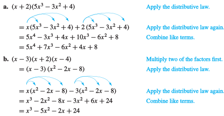
Example 8.1.

Compute the products.

\(\displaystyle (x + 2)(5x^3 - 3x^2 + 4)\)
\(\displaystyle (x - 3)(x + 2)(x - 4)\)

Solution.

diagram of polynomial multiplication

Example 8.2.

Multiply \((y + 2)(y^2 - 2y + 3)\text{.}\)

Solution.

\begin{equation*} \begin{aligned} (y+2)(y^2-2y+3) \amp= y(y^2-2y+3) + 2(y^2-2y+3) \\ \amp= y^3 - 2y^2 + 3y + 2y^2 - 4y + 6 \\ \amp= y^3 - y + 6 \end{aligned} \end{equation*}

In Example 8.1a, we multiplied a polynomial of degree 1 by a polynomial of degree 3, and the product was a polynomial of degree 4. In Example 8.1b, the product of three first degree polynomials is a third-degree polynomial. In Example 8.2, we multiplied a polynomial of degree 1 by a polynomial of degree 2, and the product was a polynomial is of degree 3. You might notice that the degree of the product is always the sum of the degrees of the factors; this is a useful property of polynomials that allows us to find the degree of a product without computing it.

Degree of a Product.

The degree of a product of nonzero polynomials is the sum of the degrees of the factors. That is,

if \(P(x)\) has degree \(m\) and \(Q(x)\) has degree \(n\) (and both \(P(x)\) and \(Q(x)\) are nonzero), then their product \(P(x)Q(x)\) has degree \(n + m\text{.}\)

Example 8.3.

Let \(P(x) = 5x^4 - 2x^3 + 6x^2 - x + 2\text{,}\) and \(Q(x) = 3x^3 - 4x^2 + 5x + 3\text{.}\)

What is the degree of their product? What is the coefficient of the lead term?
Find the coefficient of the \(x^3\)-term of the product.

Solution.

The degree of \(P\) is \(4\text{,}\) and the degree of \(Q\) is \(3\text{,}\) so the degree of their product is \(4 + 3 = 7\text{.}\) The only degree \(7\) term of the product is \((5x^4)(3x^3) = 15x^7\text{,}\) which has coefficient \(15\text{.}\)
In the product, each term of \(P(x)\) is multiplied by each term of \(Q(x)\text{.}\) We get degree \(3\) terms by multiplying together terms of degree \(0\) and \(3\text{,}\) or \(1\) and \(2\text{.}\) For these polynomials, the possible combinations are:

\(P(x)\) \(Q(x)\) Product

\(2\) \(3x^3\) \(6x^3\)

\(-2x^3\) \(3\) \(-6x^3\)

\(-x\) \(-4x^2\) \(4x^3\)

\(6x^2\) \(5x\) \(30x^3\)

The sum of the third-degree terms of the product is \(34x^3\text{,}\) with coefficient \(34\text{.}\)

Checkpoint 8.4.

Let \(f(x) = 2x^6 + 2x^4 - x^3 + 5x^2 + 1\) and \(g(x) = x^5 - 3x^4 + 2x^3 + x^2 - 4x - 2\text{.}\)

(a)

What is the degree of their product? What is the coefficient of the lead term?

(b)

Find the coefficient of the \(x^4\)-term of the product.

Subsection 8.1.2 Classifying Polynomials by Degree

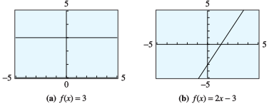
The graph of a polynomial function depends first of all on its degree. We have already studied the graphs of polynomials of degrees \(0\text{,}\) \(1\text{,}\) and \(2\text{.}\)

A polynomial of degree \(0\) is a constant, and its graph is a horizontal line. An example of such a polynomial function is \(f(x) = 3\) (see Figure 8.5a).
A polynomial of degree \(1\) is a linear function, and its graph is a straight line. The function \(f(x) = 2x - 3\) is an example of a polynomial of degree \(1\text{.}\) (See Figure 8.5b.)

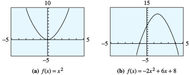
Quadratic functions, such as \(f(x) = -2x^2 + 6x + 8\text{,}\) are polynomials of degree \(2\text{.}\) The graph of every quadratic function is a parabola, with the same basic shape as the standard parabola, \(y = x^2\text{.}\) (See Figure 8.6.) Notice that the graph changes from increasing to decreasing or vice versa at one point. This point of a parabola is the same as its vertex (which we defined in section 10.2).

Subsection 8.1.3 Cubic Polynomials

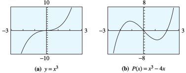
Do the graphs of all cubic , or third-degree, polynomials have a basic shape in common? We can graph a few examples and find out. Unlike the basic parabola, the graph of \(y = x^3\) is always increasing. At the origin, however, it changes from concave down to concave up. A point where the graph changes concavity is called an inflection point . You do not need to concern yourself with concavity and inflection points in this course. However, if you continue on to Calculus, this definition will appear again!

Example 8.7.

Graph the cubic polynomial \(P(x) = x^3 - 4x\) and compare its graph with that of the basic cubic, \(y = x^3\text{.}\)

Solution.

The graph of the basic cubic is shown in Figure 8.8a. To help us understand the graph of the polynomial \(P(x) = x^3 - 4x\text{,}\) we will evaluate the function to make a table of values. We can do this by hand or use the Table feature on the graphing calculator.

\(x\)	\(-3\)	\(-2\)	\(-1\)	\(0\)	\(1\)	\(2\)	\(3\)
\(P(x)\)	\(-15\)	\(0\)	\(3\)	\(0\)	\(-3\)	\(0\)	\(15\)

The graph of \(P(x) = x^3 - 4x\) is shown in Figure 8.8b. While the graph of \(P(x)\) does not look exactly like the graph of \(y=x^3\text{,}\) it is similar, especially at the edges of the graphs.

Despite the differences in the central portions of the two graphs, they exhibit similar long-run behavior.

For very large and very small values of \(x\text{,}\) both graphs look like the power function \(y = x^3\text{.}\)
The \(y\)-values increase from \(-\infty\) toward zero in the third quadrant, and they increase from zero toward \(+\infty\) in the first quadrant. Or we might say that the graphs start at the lower left and extend to the upper right.

All cubic polynomials display this behavior when their lead coefficients (the coefficient of the \(x^3\) term) are positive.

Both of the graphs in Example 8.7 are smooth curves without any breaks or holes. This smoothness is a feature of the graphs of all polynomial functions.
The domain of any polynomial function is the entire set of real numbers.

Example 8.9.

Complete the table of values below for \(C(x) = -x^3 - 2x^2 + 4x + 4\text{.}\)

\(x\)	\(-4\)	\(-3\)	\(-2\)	\(-1\)	\(0\)	\(1\)	\(2\)	\(3\)	\(4\)
\(y\)	\(\hphantom{000}\)	\(\hphantom{000}\)	\(\hphantom{000}\)	\(\hphantom{000}\)	\(\hphantom{000}\)	\(\hphantom{000}\)	\(\hphantom{000}\)	\(\hphantom{000}\)	\(\hphantom{000}\)

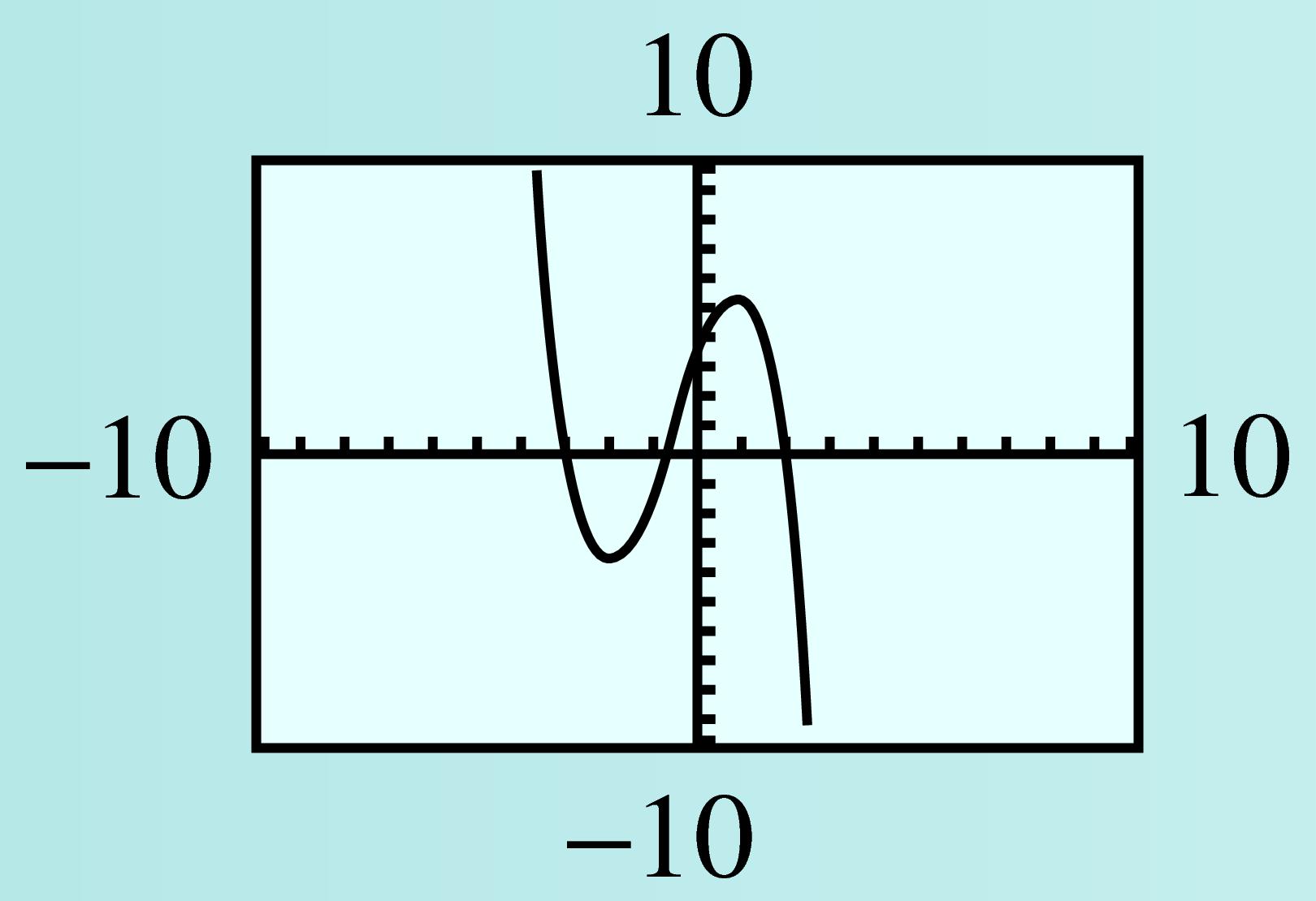
Graph \(y = C(x)\) in the standard window. Compare the graph to the graphs in Example 8.7: What similarities do you notice? What differences?

Solution.

\(x\) \(-4\) \(-3\) \(-2\) \(-1\) \(0\) \(1\) \(2\) \(3\) \(4\)

\(y\) \(20\) \(1\) \(-4\) \(-1\) \(4\) \(5\) \(-4\) \(-29\) \(-76\)
cubic

Both graphs have three \(x\)-intercepts, but the function in Example 8.7 has long-term behavior like \(y = x^3\text{,}\) and this function has long-term behavior like \(y = -x^3\text{.}\)

Subsection 8.1.4 Quartic Polynomials

Now let’s compare the long-term behavior of two quartic , or fourth-degree, polynomials.

Example 8.10.

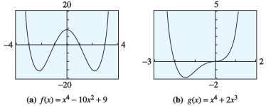
Graph the polynomials \(f(x) = x^4 - 10x^2 + 9\) and \(g(x) = x^4 + 2x^3\text{,}\) and compare.

Solution.

For each function we make a table of values.

\(x\)	\(-4\)	\(-3\)	\(-2\)	\(-1\)	\(0\)	\(1\)	\(2\)	\(3\)	\(4\)
\(f(x)\)	\(105\)	\(0\)	\(-15\)	\(0\)	\(9\)	\(0\)	\(-15\)	\(0\)	\(105\)
\(G(x)\)	\(128\)	\(27\)	\(0\)	\(-1\)	\(0\)	\(3\)	\(32\)	\(135\)	\(384\)

The graphs are shown in Figure 8.11. All the essential features of the graphs are shown in these viewing windows. The graphs continue forever in the directions indicated, without any additional twists or turns. You can see that the graph of \(f\) has three turning points, and the graph of \(g\) has one turning point.

As in Example 8.7, both graphs have similar long-term behavior. The \(y\)-values decrease from \(-\infty\) toward zero as \(x\) increases from \(-\infty\text{,}\) and the \(y\)-values increase toward \(+\infty\) as \(x\) increases to \(+\infty\text{.}\) This long-term behavior is similar to that of the power function \(y = x^4\text{.}\) Its graph also starts at the upper left and extends to the upper right.

Example 8.12.

Complete the following table of values for \(Q(x) = -x^4 - x^3 - 6x^2 + 2\text{.}\)

\(x\)	\(-4\)	\(-3\)	\(-2\)	\(-1\)	\(0\)	\(1\)	\(2\)	\(3\)	\(4\)
\(y\)	\(\hphantom{000}\)	\(\hphantom{000}\)	\(\hphantom{000}\)	\(\hphantom{000}\)	\(\hphantom{000}\)	\(\hphantom{000}\)	\(\hphantom{000}\)	\(\hphantom{000}\)	\(\hphantom{000}\)

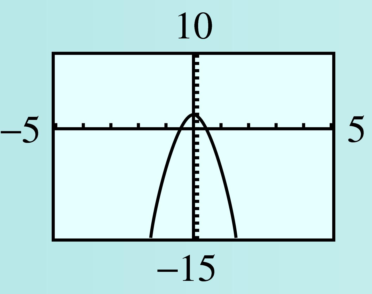
Graph \(y = Q(x)\) in the window

\begin{align*} \text{Xmin} \amp = -5 \amp\amp \text{Xmax} = 5\\ \text{Ymin} \amp = -15 \amp\amp \text{Ymax} = 10. \end{align*}

Compare the graph to the graphs in Example 8.10: What similarities do you notice? What differences?

Solution.

\(x\) \(-4\) \(-3\) \(-2\) \(-1\) \(0\) \(1\) \(2\) \(3\) \(4\)

\(y\) \(-286\) \(-106\) \(-30\) \(-4\) \(2\) \(-6\) \(-48\) \(-160\) \(-414\)
cubic

The graphs all have long-term behavior like a fourth degree power function, \(y = ax^4\text{.}\) The long-term behavior of the graphs in Example 8.10 is the same as that of \(y = x^4\text{,}\) but the graph here has long-term behavior like \(y = -x^4\text{.}\)

In the exercises, you will consider more graphs to help you verify the following observations.

Long-Run Behavior of Polynomial Functions.

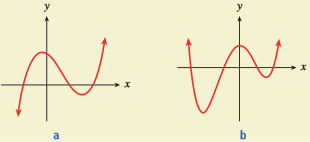
A polynomial of odd degree (with positive leading coefficient) has negative \(y\)-values for large negative \(x\)-values and positive \(y\)-values for large positive \(x\)-values. In general, this type of polynomial will have a graph similar to graph (a) below.
A polynomial of even degree (with positive leading coefficient) has positive \(y\)-values for both large positive and large negative \(x\)-values. In general, this type of polynomial will have a graph similar to graph (b) below.

graphs of a cubic and a quartic

Exercises 8.1.5 Exercises

1. Expanding Polynomial Multiplication.

a) Expand the function \(f(x) = -3 \left(x + 7\right)\left(x-2\right)\left(x-5\right)\)

\(f(x)\) =

b) What are the zeros of the function in part (a)? Enter them from smallest to largest.

\((\) , \()\) , \((\) , \()\text{,}\) \((\) , \()\)

c) What is the \(y\)-intercept?

\((\) , \()\)

Hint.

a) To expand this, we will need to multiply everything together. One way to start is to multiply the first two binomials together first, and then multiply that quadratic by the third binomial. Make sure you combine like-terms to get your final answer.

b) You are given the equation in factored form. Recall the \(x\)-intercepts occur then the output equals 0, so you can set the equation equal to 0.

c) To obtain the \(y\)-intercept, we can evaluate our answer for part (a) at \(x=0\text{.}\)

2. Identifying Polynomials.

Decide whether each of the following functions is a polynomial. If so, state the degree and leading term. If not, enter NONE in those blanks.

a) \(f(s)=5 s+4\)

Polynomial?

Yes, the given function is a polynomial
No, the given function is not a polynomial

Degree?

Leading term?

b) \(g(x)=4 x^2+x^{2.5}+x\)

Polynomial?

Yes, the given function is a polynomial
No, the given function is not a polynomial

Degree?

Leading term?

c) \(Q(t)=5 +e\cdot t^{14} +t^{3}\)

Polynomial?

Yes, the given function is a polynomial
No, the given function is not a polynomial

Degree?

Leading term?

Hint.

Recall a polynomial is a function that can be written in the form \(y=a_nx^n+a_{n-1}x^{n-1}+\cdots+a_1x^1+a_0\text{,}\) where the coefficients are constants. Note that the exponents must be non-negative whole numbers.

Look at each of the given equations and determine if it satisfies this definition.

The degree of a polynomial is the value of the largest exponent and the leading term is the term (the power function) with that largest exponent. In the above example, the degree is \(n\) and the leading term is \(a_nx^n\text{.}\)

3. Long-Run Behavior.

For each of the polynomials below, state the degree and the number of nonzero terms, and select the options that describe the long-run behavior.

a) \(p(x)=(x+5)(x-3)(3 x+1)\)

Degree:

Number of nonzero terms:

Long-run behavior:

As \(x\) goes to negative \(\infty\text{,}\) \(p(x)\) goes to positive \(\infty\text{.}\)
As \(x\) goes to negative \(\infty\text{,}\) \(p(x)\) goes to negative \(\infty\text{.}\)
As \(x\) goes to positive \(\infty\text{,}\) \(p(x)\) goes to negative \(\infty\text{.}\)
As \(x\) goes to positive \(\infty\text{,}\) \(p(x)\) goes to positive \(\infty\text{.}\)

b) \(q(x)=4.6 x^3+12 x- 3 x^{6}\)

Degree:

Number of nonzero terms:

Long-run behavior:

As \(x\) goes to positive \(\infty\text{,}\) \(q(x)\) goes to negative \(\infty\text{.}\)
As \(x\) goes to positive \(\infty\text{,}\) \(q(x)\) goes to positive \(\infty\text{.}\)
As \(x\) goes to negative \(\infty\text{,}\) \(q(x)\) goes to negative \(\infty\text{.}\)
As \(x\) goes to negative \(\infty\text{,}\) \(q(x)\) goes to positive \(\infty\text{.}\)

c) \(v(x)=x^2-7x^2+ 3 x^4+1\)

Degree:

Number of nonzero terms:

Long-run behavior:

As \(x\) goes to positive \(\infty\text{,}\) \(v(x)\) goes to negative \(\infty\text{.}\)
As \(x\) goes to positive \(\infty\text{,}\) \(v(x)\) goes to positive \(\infty\text{.}\)
As \(x\) goes to negative \(\infty\text{,}\) \(v(x)\) goes to negative \(\infty\text{.}\)
As \(x\) goes to negative \(\infty\text{,}\) \(v(x)\) goes to positive \(\infty\text{.}\)

d) \(w(x)=- 5 x^{5}\)

Degree:

Number of nonzero terms:

Long-run behavior:

As \(x\) goes to positive \(\infty\text{,}\) \(w(x)\) goes to positive \(\infty\text{.}\)
As \(x\) goes to negative \(\infty\text{,}\) \(w(x)\) goes to negative \(\infty\text{.}\)
As \(x\) goes to positive \(\infty\text{,}\) \(w(x)\) goes to negative \(\infty\text{.}\)
As \(x\) goes to negative \(\infty\text{,}\) \(w(x)\) goes to positive \(\infty\text{.}\)

Hint.

Recall the degree of a polynomial is the value of the largest exponent and the leading term is the term (the power function) with that largest exponent. A nonzero term is a term that has a nonzero coefficient. For example, \(0x^2\) is not a nonzero term, but \(3x^2\) is a nonzero term.

The polynomial will "act like" it’s leading term in its long-run behavior. To answer this part of the question, you should determine the leading term and it’s long-run behavior.

4. Comparing Polynomial Functions.

Graph each of the following polynomials on your own piece of paper or using graphing software like Desmos. What is similar about them? What is different? For each of these questions, select all that apply.

a) \(f(x) = 4 x^{4} + 3 x - 3\)

b) \(g(x) = 4 x^{4} + 2x\)

c) \(h(x) = 4 x^{4} + 5\)

What is similar?

For each, as \(x\) goes to \(+ \infty\text{,}\) the function goes to \(+\infty\text{.}\)
They are all degree 4 polynomials.
They all have a leading coefficient of 4.
For each, as \(x\) goes to \(- \infty\text{,}\) the function goes to \(+\infty\text{.}\)
For each, as \(x\) goes to \(- \infty\text{,}\) the function goes to \(-\infty\text{.}\)
For each, as \(x\) goes to \(+ \infty\text{,}\) the function goes to \(-\infty\text{.}\)
They all have 2 terms
They all have only one \(x\)-intercept.

What is different?

They have a different number of terms.
They have different \(y\) intercepts.
They have different \(x\)-intercepts.
They have different leading coefficients.
They are different degree polynomials.
They have different long-run behaviors.

Hint.

Make sure you graph the functions to get all of the possible answers.

You should also compare the equations themselves.

5. Properties of Polynomials.

Water is pumped into a cylindrical tank, and then drained out. Suppose the volume of water in the tank in cubic meters after \(t\) hours is given by the equation

\begin{equation*} V(t)=-0.064t^3+0.256t^2-0.836 t+7. \end{equation*}

Using an online tool like Desmos, sketch a graph of \(V(t)\) on the interval \([0,8]\text{.}\)

a) Find and interpret the maximum value of \(V(t)\) on this interval.

Maximum value:

cubic feet
feet
hours

We can interpret this as:

the fastest the water is draining at any time in the given time interval is 7 feet per second.
the amount of time it takes for all of the water to drain from the tank is 7 hours.
the most water in the tank at any time in the given time interval is the initial amount.
the height of the tank in feet is 7 feet.

b) Interpret both the vertical and horizontal intercepts of \(V(t)\) in the context of the problem.

The vertical intercept:

is the amount of water left in the tank after 7 hours.
is the initial volume of water in the tank.
is the fastest speed at which the water is draining from the tank.
is the amount of time it takes for all of the water to drain from the tank.

The horizontal intercept:

is the duration of time in hours it takes for all of the water to drain from the tank.
is the fastest speed at which the water is draining from the tank.
is the initial volume of water in the tank.
is the amount of water left in the tank after 7 hours.

Hint.

Make sure to look at the graph on the specified domain.

To determine the interpretations, think about what units are associated with the input and output values.

6. Properties of Polynomials.

Let \(f(x)\) be a polynomial function of degree \(n\text{,}\) where \(n\) is a positive integer.

a) Suppose \(n\) is even. Are the following statements true or false for every polynomial of degree \(n\text{?}\) If true, select "NONE" from the list of possible counterexamples. If false, select all functions that are counterexamples to the statement.

i) \(f(x)\) is an invertible function.

True
False

\(\displaystyle x^2 + 4x + 3\)
\(\displaystyle -x^4 -5x +3\)
\(\displaystyle -x^3\)
\(\displaystyle x^5 -5x +3\)
\(\displaystyle -x +3\)
NONE

ii) If \(\displaystyle \lim_{x\to -\infty} f(x) = -\infty\text{,}\) then \(\displaystyle \lim_{x\to \infty} f(x)=-\infty\text{.}\)

True
False

\(\displaystyle x^2 + 4x + 3\)
\(\displaystyle -x^4 -5x +3\)
\(\displaystyle -x^3\)
\(\displaystyle x^5 -5x +3\)
\(\displaystyle -x +3\)
NONE

iii) \(\displaystyle \lim_{x\to \infty} f(x) = -\infty\)

True
False

\(\displaystyle x^2 + 4x + 3\)
\(\displaystyle -x^4 -5x +3\)
\(\displaystyle -x^3\)
\(\displaystyle x^5 -5x +3\)
\(\displaystyle -x +3\)
NONE

b) Suppose \(n\) is odd. Are the following statements true or false for every polynomial of degree \(n\text{?}\) If true, select "NONE" from the list of possible counterexamples. If false, select all functions that are counterexamples to the statement.

i) \(f(x)\) is an invertible function.

True
False

\(\displaystyle x^2 + 4x + 3\)
\(\displaystyle -x^4 -5x +3\)
\(\displaystyle -x^3\)
\(\displaystyle x^5 -5x +3\)
\(\displaystyle -x +3\)
NONE

ii) If \(\displaystyle \lim_{x\to \infty} f(x) = \infty\text{,}\) then \(\displaystyle \lim_{x\to -\infty} f(x)=-\infty\text{.}\)

True
False

\(\displaystyle x^2 + 4x + 3\)
\(\displaystyle -x^4 -5x +3\)
\(\displaystyle -x^3\)
\(\displaystyle x^5 -5x +3\)
\(\displaystyle -x +3\)
NONE

iii) \(\displaystyle \lim_{x\to \infty} f(x) = \infty\)

True
False

\(\displaystyle x^2 + 4x + 3\)
\(\displaystyle -x^4 -5x +3\)
\(\displaystyle -x^3\)
\(\displaystyle x^5 -5x +3\)
\(\displaystyle -x +3\)
NONE

Hint.

It may be useful to think about whether the statement is true for each of the given options in the lists below the drop-down menus. If the statement is not true for at least one of the options, it can’t be true in general.

For a statement to be true, it must not fail for any polynomial function \(f(x)\) of degree \(n\text{.}\)

Prev Top Next

\(P(x)\)	\(Q(x)\)	Product
\(2\)	\(3x^3\)	\(6x^3\)
\(-2x^3\)	\(3\)	\(-6x^3\)
\(-x\)	\(-4x^2\)	\(4x^3\)
\(6x^2\)	\(5x\)	\(30x^3\)