Section 7.2 Power Functions

Supplemental Videos.

The main topics of this section are also presented in the following videos:

Power Functions

Before we begin discussing the behavior of power functions, it is important that we remember our laws of exponents. Recall that a positive integer exponent tells us how many times its base occurs as a factor in an expression. For example,

\begin{equation*} 4a^3b^2 \text{ means } 4aaabb. \end{equation*}

Recall too the definition of a negative, zero, or non-integer exponent:

Definition of Negative, Zero, and Rational Exponents.

\begin{equation*} \begin{aligned} a^{-n} \amp = \frac{1}{a^n} \amp\amp (a \ne 0) \\ a^0 \amp = 1 \amp\amp (a \ne 0) \\ a^{\frac{p}{q}} \amp = \sqrt[q]{a^p} \amp\amp (a \ne 0) \end{aligned} \end{equation*}

The most common example of a non-integer power is \(a^{\frac{1}{2}} = \sqrt{a}\text{.}\)

As we begin combining both positive and negative exponents, we adhere to the following rules:

Laws of Exponents.

\(\displaystyle \displaystyle{a^m\cdot a^n = a^{m+n}}\)
\(\displaystyle \displaystyle{\frac{a^m}{a^n}=a^{m-n}}\)
\(\displaystyle \displaystyle{\left(a^m\right)^n=a^{mn}}\)
\(\displaystyle \displaystyle{\left(ab\right)^n=a^n b^n}\)
\(\displaystyle \displaystyle{\left(\frac{a}{b}\right)^n=\frac{a^n}{b^n}}\)

Example 7.3.

\begin{align*} \text{a}\amp. ~x^3\cdot x^{-5} = x^{3-5} = x^{-2} \amp\amp \text{Apply the first law: Add exponents.}\\ \text{b}\amp. ~\frac{8x^{-2}}{4x^{-6}}= \frac{8}{4}x^{-2-(-6)} = 2x^4 \amp\amp \text{Apply the second law: Subtract exponents.}\\ \text{c}\amp. ~\left(5x^{-3}\right)^{-2}= 5^{-2}(x^{-3})^{-2}=\frac{x^6}{25} \amp\amp \text{Apply laws IV and III.} \end{align*}

You can check that each of the calculations in Example 7.3 is shorter when we use negative exponents instead of converting the expressions into algebraic fractions.

Example 7.4.

Simplify by applying the laws of exponents.

\(\displaystyle \left(2a^{-4}\right) \left(-4a^2\right)\)
\(\displaystyle \dfrac{(r^2)^{-3}}{3r^{-4}}\)

Solution.

\(\displaystyle (2a^{-4})(-4a^2)=-8a^{-4+2}=-8a^{-2}=\dfrac{-8}{a^2} \)
\(\displaystyle \dfrac{(r^2)^{-3}}{3r^{-4}}=\dfrac{r^{-6}}{3r^{-4}}=\dfrac{1}{3r^2} \)

Caution 7.5.

The laws of exponents do not apply to sums or differences of powers. We can add or subtract like terms, that is, powers of the same variable with the same exponent. For example,

\begin{equation*} 6x^{-2} + 3x^{-2} = 9x^{-2} \end{equation*}

but we cannot add or subtract terms with different exponents. Thus, for example,

\begin{align*} 4x^2 \amp- 3x^{-2} \amp\amp \text{cannot be simplified, and}\\ x^{-1} \amp + x^{-3}\amp\amp \text{cannot be simplified}. \end{align*}

Subsection 7.2.1 Power Functions

Power Function.

A function of the form

\begin{equation*} f(x) = k(x)^p \end{equation*}

where \(k\) is a nonzero constant and \(p\) is any constant, is called a power function . In particular, if \(p=0\text{,}\) then \(f(x)\) is the constant function \(f(x) = k\text{.}\)

Examples of power functions are

\begin{equation*} V(r ) = \frac{4}{3}\pi (r)^3 ~~\text{ and }~~L(T ) = 0.8125(T)^2. \end{equation*}

In addition, the basic functions

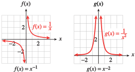
\begin{equation*} f (x) = \frac{1}{x} ~~\text{ and }~~ g(x) = \frac{1}{x^2} \end{equation*}

can be written as

\begin{equation*} f (x) = x^{-1} ~~\text{ and }~~ g(x) = x^{-2}. \end{equation*}

Their graphs are shown in Figure 7.6. Note that the domains of power functions with negative exponents do not include zero.

described in detail following the image — Figure 7.6.

Example 7.7.

Which of the following are power functions?

\(\displaystyle f (x) = \dfrac{1}{3}x^4 + 2\)
\(\displaystyle g(x) = \dfrac{1}{3x^4}\)
\(\displaystyle h(x) = \dfrac{x + 6}{x^3}\)

Solution.

This is not a power function, because of the addition of the constant term.
We can write \(g(x) = \frac{1}{3}x^{-4}\text{,}\) so \(g\) is a power function.
This is not a power function, but it can be treated as the sum of two power functions, because \(h(x) = x^{-2} + 6x^{-3}\text{.}\)

Example 7.8.

Write each function as a power function in the form \(y = kx ^p\text{.}\)

\(\displaystyle f (x) = {12}{x^2}\)
\(\displaystyle g(x) = \dfrac{1}{4x}\)
\(\displaystyle h(x) = \dfrac{2}{5x^6}\)

Solution.

\(\displaystyle f (x) = 12x^{-2}\)
\(\displaystyle g(x)=\dfrac{1}{4}x^{-1} \)
\(\displaystyle h(x)=\dfrac{2}{5}x^{-6} \)

Subsection 7.2.2 Long Run Behavior

While power functions do not in general have to have integer exponents, these will be the types of power functions we are most interested in. In particular, we will look at the graphs and long run behavior of power functions with integer exponents. By long run behavior of a function we mean the value the function approaches as the input \(x \) goes to infinity or negative infinity.

Example 7.9.

Recall that the graph of \(f(x)=\frac{1}{x}\) and \(g(x)=\frac{1}{x^2}\) are given by:

Identify the long run behavior of each of these functions.

Solution.

Let’s begin with the long run behavior of \(f(x) \text{.}\) Looking at the graph, we see that as \(x \) goes to infinity (i.e. as we move farther to the right on the \(x \)-axis) the output values of \(f(x)\) are getting close to 0. Similarly, as \(x \) goes to negative infinity (as we move farther to the left on the \(x\)-axis) the output values of \(f(x)\) are also getting closer to 0. We write this as

\begin{equation*} \text{as}\ \ x\to\pm\infty\ \ f(x)\to 0\text{.} \end{equation*}

By identical reasoning as above, we also have that

\begin{equation*} \text{as}\ \ x\to\pm\infty\ \ g(x)\to 0\text{.} \end{equation*}

In general, we have the following behaviors of power functions with integer exponents:

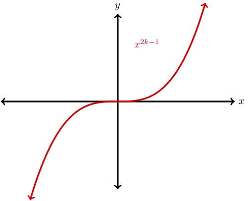
The graph of

\begin{equation*} y=x^\text{(odd positive number)} \end{equation*}

is shown to the right. The long run behavior of such a function is given by

\begin{align*} x^\text{(odd positive number)}\to -\infty\ \amp \text{as}\ x\to -\infty\ ,\ \ \text{and}\\ x^\text{(odd positive number)}\to \infty\ \amp \text{as}\ x\to \infty. \end{align*}

Examples of such functions are \(x,x^3,x^5,\) etc.

graphs positive odd powers

Figure 7.11.
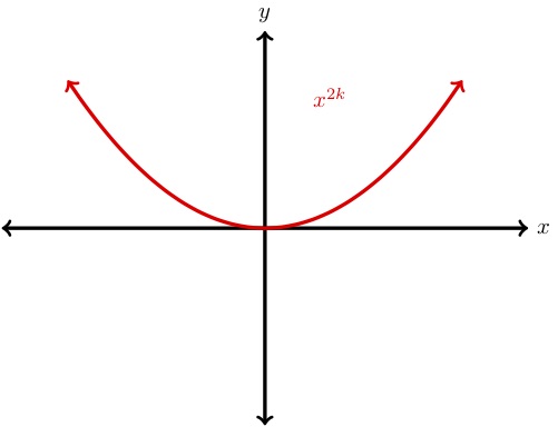
The graph of

\begin{equation*} y=x^\text{even positive number} \end{equation*}

is shown to the right. The long run behavior of such a function is given by

\begin{align*} x^\text{even positive number}\to \infty\ \amp \text{as}\ x\to \pm\infty. \end{align*}

Examples of such functions are \(x^2,x^4,x^6,\) etc.

graphs positive even powers

Figure 7.12.
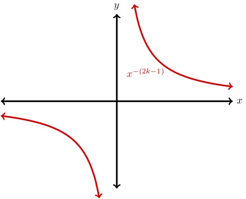
The graph of

\begin{equation*} y=x^\text{odd negative number} \end{equation*}

is shown to the right. The long run behavior of such a function is given by

\begin{align*} x^\text{odd negative number}\to 0\ \amp \text{as}\ x\to \pm\infty. \end{align*}

Examples of such functions are \(x^{-1},x^{-3},x^{-5},\) etc.

graphs negative odd powers

Figure 7.13.
The graph of

\begin{equation*} y=x^\text{even negative number} \end{equation*}

is shown to the right. The long run behavior of such a function is given by

\begin{align*} x^\text{even negative number}\to 0\ \amp \text{as}\ x\to \pm\infty \end{align*}

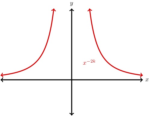
Examples of such functions are \(x^{-2},x^{-4},x^{-6},\) etc.

graphs negative even powers

Figure 7.14.

Exercises 7.2.3 Exercises

1. Simplifying Exponents.

Simplify the expression \(4t^{4}(2t^{1/5})^{2}\text{.}\)

Hint.

To simplify the expression \(4t^{4}(2t^{1/5})^{2}\text{,}\) we need to combine the coefficients and the exponents. Recall that \((b^n)^m=b^{n\cdot m}\text{,}\) \((a\cdot b)^m=a^mb^m\text{,}\) and \(t^m t^n=t^{m+n}\text{.}\)

The goal is to combine all constant pieces and all exponents together to simplify the expression. You should end up with something of the form \(kt^p\text{,}\) where \(k\) and \(p\) are constants.

2. Identifying Power Functions.

Ohm’s law states that as the resistance in a circuit, \(R\) (measured in ohms), is increased, the electrical current flowing in the circuit, \(I\) (measured in amperes, or amps), decreases. In particular, \(I(R)=V/R\text{,}\) where here \(V\) represents a constant voltage value.

a) Is \(I(R)\) a power function? If yes, identify \(k\) and \(p\text{.}\) If not, please enter "NONE" in both spaces.

\(k=\)

\(p=\)

b) If the current flowing in a circuit is 0.018 amps when the resistance is 600 ohms, what is the current when the resistance is 700 ohms?

Hint.

a) Try to rewrite the equation in the form \(y=kR^p\text{,}\) where \(k\) and \(p\) are constants. If you can, then this is a power function. Otherwise, it is not.

b) Since we are given that the current flowing in a circuit is 0.018 amps when the resistance is 600 ohms, we have that

\begin{equation*} 0.018=\frac{V}{600}. \end{equation*}

You should use this information to solve for the constant \(V\text{.}\)

Then you can plug in the new given resistance to find the answer.

3. Identifying Power Functions.

Determine whether the following functions are power functions. If yes, identify the values of \(k\) and \(p\text{.}\) If not, write "NONE" for both \(k\) and \(p\text{.}\)

a) \(g(t) = \ln(x^{5})\)

i) Is \(g(x)\) a power function?

ii) \(k=\)

iii) \(p=\)

b) \(C(x) = \dfrac{9}{10 \sqrt[3]{x}}\)

i) Is \(C(x)\) a power function?

ii) \(k=\)

iii) \(p=\)

c) \(P(x) = 8x^2+3x^2\)

i) Is \(P(x)\) a power function?

ii) \(k=\)

iii) \(p=\)

d) \(k(x) = \ln(5^x)\)

i) Is \(k(x)\) a power function?

ii) \(k=\)

iii) \(p=\)

4. Graphs of Power Functions.

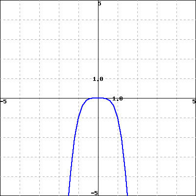
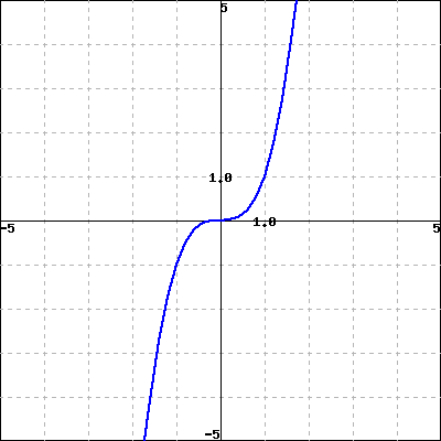
Determine whether the following power functions have odd or even powers.

Even
Odd

Even
Odd

Hint.

Think back to the definition of even and odd function from the chapter on Function Transformations: https://mathbooks.unl.edu/PreCalculus/The-Natural-Base.html

The exponent of a power function ends up relating to these concepts in an intuitive way.

5. End Behavior of Power Functions.

Determine the following long-run behaviors. Please use "INF" for positive infinity and "-INF" for negative infinity. If the long run behavior is a number, please enter that number in the blank.

a) As \(x \to \infty\text{,}\) \(-10x^{-2}+5 \to\)

b) As \(x \to -\infty\text{,}\) \(7x^{-7} \to\)

c) As \(x \to \infty\text{,}\) \(8x^{2} \to\)

d) As \(x \to \infty\text{,}\) \(5x^{-6}+3 \to\)

Hint.

One way to tackle this problem is to plug in large positive or negative values, based on whether you are looking at \(\infty\) or \(-\infty\text{.}\)

Another way is to sketch a graph of the function to see the end-behavior.

6. Writing Power Functions.

Find a power function, \(f(x)\text{,}\) satisfying the following.

a) The points \((2,2)\) and \(\left(\dfrac{1}{3},\dfrac{1}{18}\right)\) lie on the graph of \(f(x)\text{.}\)

\(f(x)=\)

\(x\)	2	3	5
\(f(x)\)	64	486	6250

\(f(x)=\)

Hint.

a) For the first part, we need to find a formula for \(f(x)=kx^p\) that goes through the points \((2,2)\) and \(\left(\dfrac{1}{3},\dfrac{1}{18}\right)\text{.}\) We can set up two equations:

\begin{equation*} 2=k(2)^p \end{equation*}

and

\begin{equation*} \frac{1}{18}=k\left(\frac{1}{3}\right)^p. \end{equation*}

We can divide these two equations to get the following:

\begin{equation*} \frac{2}{1/18}=\frac{k(2)^p}{k(1/3)^p}. \end{equation*}

From here you need to solve for the value of \(p\) using exponent rules and logarithms. Recall that when we divide by a fraction, we can multiply by the reciprocal to simplify. We also need that \(\dfrac{a^p}{b^p}=\left(\dfrac{a}{b}\right)^p\text{.}\)

Once you solve for \(p\text{,}\) you can use either of the initial equations to find the value of \(k\) to write your equation.

b) We will use an identical method to find the formula for \(f(x)\) in part b. We can set up two formulas:

\begin{equation*} 64=k(2)^p \end{equation*}

and

\begin{equation*} 486=k(3)^p. \end{equation*}

7. Application of Power Functions.

The Deepwater Horizon oil spill began on April 20, 2010, and the well was not declared sealed until September of 2010. Suppose that the spill was relatively circular in shape, and that the radius of the spill increased at a rate of approximately \(6\) miles per day.

a) Fill in the table below showing the radius in miles, \(r\text{,}\) of the oil spill \(t\) days after April 20.

\(t\)	0	2	4	6
\(r\)

b) Write a formula for \(r\) as a function of \(t\text{.}\)

\(r(t)=\)

c) Venice, Louisiana is approximately 50 miles from the site of the well. Approximately how long did it take for oil to wash up on the shores of Venice? Please round your answer up to the next whole number.

days

d) Assuming the spill was circular, write a formula for the area, \(A\text{,}\) of the oil spill as a function of \(t\text{.}\) Hint: recall that the area of a circle is given by \(\pi r^2\text{.}\)

\(A(t)=\)

e) How many full days after the initial spill would it take to guarantee the area of the spill was 6000 square miles? Please round your answer up to the next whole number.

days

Hint.

a) Since the radius of the oil spill increased at a rate of 6 miles per day, starting at a radius of 0, we can multiply the number of days by the rate 6 per day to get the radius after \(t\) days.

b) Using what we found in part a), we see that this is a linear function (it is increasing by a fixed constant each day). Determine the slope and vertical intercept to write the equation.

c) Since Venice, Louisiana is approximately 50 miles from the site of the well, we want to set \(r(t)\) equal to 50 and solve for \(t\text{.}\) Make sure you round to the next full day.

d) If we assume the spill was circular, to find a formula for the area, we want to compose the area function, \(A(r)=\pi r^2\text{,}\) with the function that gives us the radius \(t\) days after the spill began. Think about what function gives you the radius.

e) Finally, to find how long it takes for the area of the spill to reach 6000 square miles, we want to set 6000 equal to the equation for \(A(t)\) and solve for \(t\text{.}\)

Prev Top Next