Josh Brummer, Taran Funk, Lawrence Seminario-Romero, Ariel Setniker, Karina Uhing, Nathan Wakefield, Catherine Zimmitti, The Mabel Elizabeth Kelly Fund
In this section we will explore the invertibility of a function. In other words, by the end of this section we will be able to test if a function is invertible.
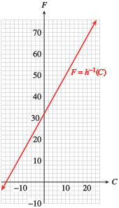
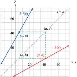
In Example 2.25, we used a graph of \(h\) to read values of \(h^{-1}\text{.}\) But we can also plot the graph of \(h^{-1}\) itself. Because \(C\) is the input variable for \(h^{-1}\text{,}\) we plot \(C\) on the horizontal axis and \(F\) on the vertical axis. To find some points on the graph of \(h^{-1}\text{,}\) we interchange the coordinates of points on the graph of \(h\text{.}\) The graph of \(h^{-1}\) is shown in Figure 4.1.
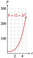
The Park Service introduced a flock of \(12\) endangered pheasant into a wildlife preserve. After \(t\) years, the population of the flock was given by
\begin{equation*}
P = f (t) = 12 + 2t^3.
\end{equation*}
Graph the function on the domain \([0, 5]\text{.}\)
We solve \(P = 12 + 2t^3\) for \(t\) in terms of \(P\text{.}\)
\begin{align*}
2t^3 \amp = P - 12\amp\amp\text{Subtract 12 from both sides.}\\
t^3 \amp = \frac{P - 12}{2}\amp\amp\text{Divide both sides by 2.}\\
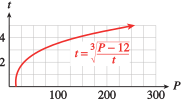
t \amp = \sqrt[3]{\frac{P - 12}{2}}\amp\amp\text{Take cube roots.}
\end{align*}
The inverse function is \(t = f^{-1}(P) =\sqrt[3]{\dfrac{P - 12}{2}}\text{.}\) It tells us the number of years it takes for the pheasant population to grow to size \(P\text{.}\)
The formula \(T = f(L) = 2\pi \sqrt{\dfrac{L}{32}}\) gives the period in seconds, \(T\text{,}\) of a pendulum as a function of its length in feet, \(L\text{.}\)
We can always find the inverse of a function \(y=f(x) \) simply by solving for \(x \) thus interchanging the role of the input and output variables. In the preceding examples, this process created a new function. However, this process does not always lead to be a function.
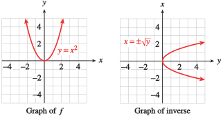
For example, to find the inverse of \(y = f (x) = x^2\text{,}\) we solve for \(x\) to get \(x = \pm\sqrt{y}\text{.}\) When we regard \(y\) as the input and \(x\) as the output, the relationship does not describe a function. This can be seen as plugging in \(y=4 \text{,}\) for example, gives two outputs \(x=2 \) and \(x=-2\text{.}\) The graphs of \(f\) and its inverse are shown in Figure 4.6. (Note that for the graph of the inverse, we plot \(y\) on the horizontal axis and \(x\) on the vertical axis.) Because the graph of the inverse does not pass the vertical line test, it is not a function.
For many applications, it is important to know whether or not the inverse of \(f\) is a function. This can be determined from the graph of \(f\text{.}\) When we interchange the roles of the input and output variables, horizontal lines of the form \(y = k\) become vertical lines.
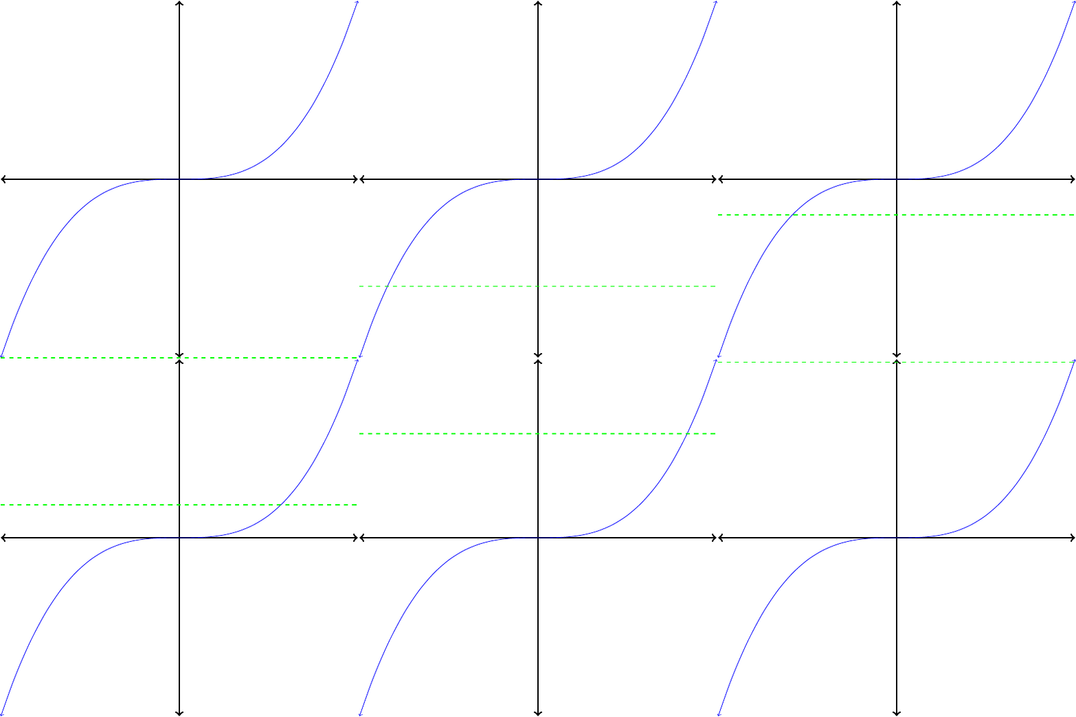
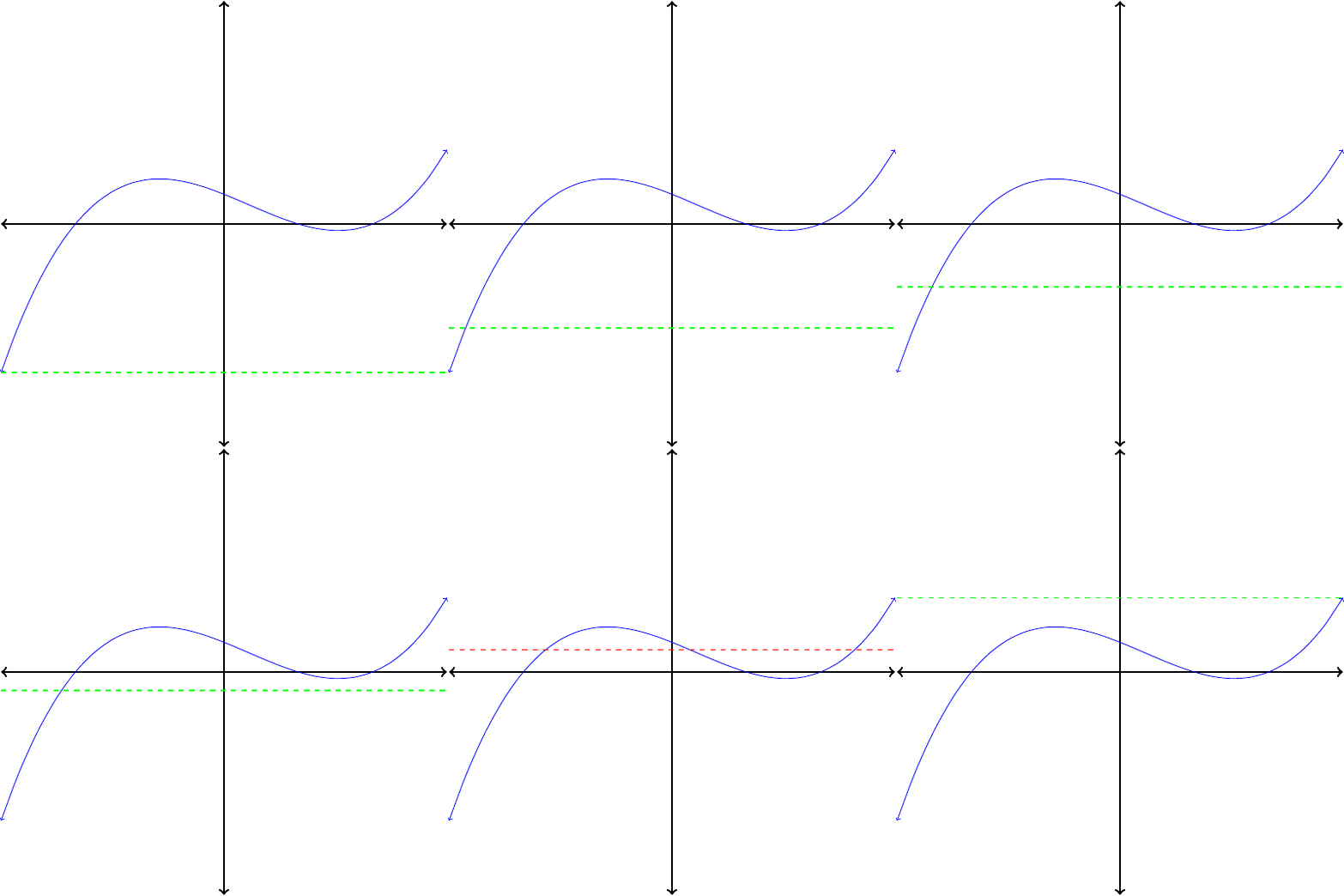
Thus, if the graph of the inverse is going to pass the vertical line test, the graph of the original function must pass the horizontal line test , namely, that no horizontal line should intersect the graph in more than one point. Notice that the graph of \(f(x) = x^2\) does not pass the horizontal line test, so we would not expect its inverse to be a function.
Figure4.7.Notice that as the line moves up the \(y-\) axis, it only ever intersects the graph in a single place. This means this function is invertible.
Figure4.8.Notice that as the line moves up the \(y-\) axis, it sometimes intersects the graph in more than one place. This means this function is not invertible.
We have been talking about how to tell if the inverse of a function is also a function, but in practice this is not the language typically used. Usually we ask this same question in the form "Is the function invertible?" The following definition explains this relationship:
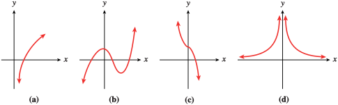
In each case, apply the horizontal line test to determine whether the function is invertible. Because no horizontal line intersects their graphs more than once, the functions pictured in Figures 4.10(a) and (c) are invertible. The functions in Figures 4.10(b) and (d) are not invertibe.
Subsection4.1.3Mathematical Properties of the Inverse Function
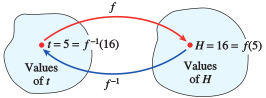
The inverse function \(f^{-1}\) undoes the effect of the function \(f\text{.}\) In Example 2.16, the function \(f(t) = 6 + 2t\) multiplies the input by \(2\) and then adds \(6\) to the result. The inverse function \(f^{-1}(H) = \dfrac{H -6}{2}\) undoes those operations in reverse order: It subtracts \(6\) from the input and then divides the result by \(2\text{.}\)
If we apply the function \(f\) to a given input value and then apply the function \(f^{-1}\) to the output from \(f\text{,}\) the end result will be the original input value. For example, if we choose \(t = 5\) as an input value, we find that
\begin{align*}
f(\alert{5})\amp= 6 + 2(\alert{5}) = \blert{16}\amp\amp\text{ Multiply by 2, then add 6.}\\
\text{and } f^{-1}(\blert{16}) \amp = \frac{\blert{16} - 6}{2} = \alert{5}.\amp\amp\text{Subtract 6, then divide by 2.}
\end{align*}
Example 4.12 illustrates the fact that if \(f^{-1}\) is the inverse function for \(f\text{,}\) then \(f\) is also the inverse function for \(f^{-1}\text{.}\)
Example 4.13 illustrates finding an inverse of a function. The general process is to move operations (or undo them) so the input variable (\(x\)) is what is alone on one side of the equation.
So far we have been careful to keep track of the input and output variables when we work with inverse functions. This is important when we are dealing with applications; the names of the variables are usually chosen because they have a meaning in the context of the application, and it would be confusing to change them.
However, we can also study inverse functions purely as mathematical objects. There is a relationship between the graph of a function and the graph of its inverse that is easier to see if we plot them both on the same set of axes.
A graph does not change if we change the names of the variables, so we can let \(x\) represent the input for both functions, and let \(y\) represent the output. Consider the function \(C = h(F)\) from Example 2.25, and its inverse function, \(F = h^{-1}(C)\text{.}\) The formulas for these functions are
\begin{align*}
C \amp = h(F) = \frac{5}{9}(F - 32)\\
F \amp = h^{-1}(C) = 32 + \frac{9}{5}C.
\end{align*}
But their graphs are the same if we write them as
\begin{align*}
y \amp = h(x) =\frac{5}{9}(x - 32)\\
y \amp= h^{-1}(x) = 32 + \frac{9}{5}x.
\end{align*}
Now, for every point \((a, b)\) on the graph of \(f\text{,}\) the point \((b, a)\) is on the graph of the inverse function. Observe in Figure 4.14 that the points \((a, b)\) and \((b, a)\) are always located symmetrically across the line \(y=x\text{.}\) The graphs are symmetric about the line \(y=x\), which means that if we were to place a mirror along the line \(y=x\text{,}\) each graph would be the reflection of the other.
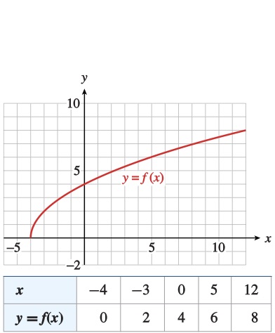
The graph of \(f\) has the same shape as the graph of \(y = \sqrt{x}\text{,}\) shifted \(4\) units to the left and stretched vertically by a factor of \(2\text{.}\)Figure 4.16a shows the graph of \(f\text{,}\) along with a table of values. By interchanging the rows of the table, we obtain points on the graph of the inverse function, shown in Figure 4.16b.
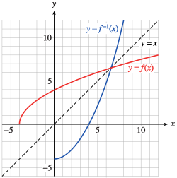
If we use \(x\) as the input variable for both functions, and \(y\) as the output, we can graph \(f\) and \(f^{-1}\) on the same grid, as shown in Figure 4.17. The two graphs are symmetric about the line \(y = x\text{.}\)
Suppose a company’s profit is a linear function of the number of units of their product that are sold. Selling 4,000 units yields a profit of $16200, and selling 6,000 units yields a profit of $22200.
Consider the following functions. Match the function to its inverse (if the inverse is one of the other functions). If the function has no inverse or if the inverse is not one of the other functions, select N/A.
A rock is dropped into the ocean from a boat. The depth, in feet, of the rock at time \(t\) can be modeled by \(d = D(t)=- 8 t^2+224 t\) for \(0\leq t\leq 14\text{,}\) where \(t\) is time in minutes since the rock entered the water.
a) Suppose the temperature of the water, \(F=T(d)\text{,}\) in degrees Fahrenheit, is decreasing exponentially as a scuba diver descends on a dive to the bottom of the ocean, where \(d\) is her depth in feet below the surface of the water. In particular, \(T(0)=85\text{,}\) and \(T(360)=72\text{.}\)
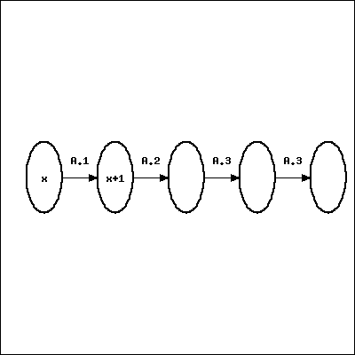
Let \(y = f(x) = 6\sqrt{x+1}-4\text{.}\) When we are computing what happens to \(x\text{,}\) we first add 1 to \(x\text{,}\) then take the square root, and so on. Represent this chain of computations visually by labeling the arrows in the diagram below. (In the possible answers below, let ’?’ be the result from the previous step.)