Section 3.2 Comparing Exponential and Linear Growth

Supplemental Videos.

The main topics of this section are also presented in the following videos:

Subsection 3.2.1 Exponential Growth

Consider the function

\begin{equation*} P(t) = 100 \cdot 3^t \end{equation*}

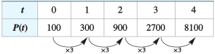
describing the population, $P\text{,}$ of a bacteria after t minutes. We say a function has exponential growth if during each time interval of a fixed length, the population is multiplied by a certain constant amount call the growth factor . Consider the table:

table of bacteria population

We can see that the bacteria population grows by a factor of $3$ each day. For this reason, we say that $3$ is the growth factor for the function. Functions that describe exponential growth can be expressed in a standard form.

Exponential Growth.

The function

\begin{equation*} P(t) = a (b)^t \end{equation*}

models exponential growth.

$a = P(0)$ is the initial value or principal value of $P\text{;}$

$b$ is the growth factor .

For the bacteria population, we have

\begin{equation*} P(t) = 100 \cdot 3^t \end{equation*}

so $a = 100$ and $b = 3\text{.}$

Example 3.4.

A colony of bacteria starts with $300$ organisms and doubles every week.

Write a formula for the population of the bacteria colony after $t$ weeks.
How many bacteria will there be after $8$ weeks? After $5$ days?

Solution.

The initial value of the population was $a = 300\text{,}$ and its weekly growth factor is $b = 2\text{.}$ Thus, a formula for the population after $t$ weeks is

\begin{equation*} P(t) = 300 \cdot 2^t. \end{equation*}
After $8$ weeks, the population will be

\begin{equation*} P(8) = 300 \cdot 2^8 = 76,800 \text{ bacteria}. \end{equation*}

Because $5$ days is $\frac{5}{7}$ of a week, after $5$ days the population will be

\begin{equation*} P\left(\frac{5}{7}\right)= 300 \cdot 2^{5/7} = 492.2. \end{equation*}

We cannot have a fraction of a bacterium, so we round to the nearest whole number, $492\text{.}$

Caution 3.5.

In Example 3.4a, note that

\begin{equation*} 300 \cdot 2^8 \ne 600^8. \end{equation*}

According to the order of operations, we compute the power $2^8$ first, then multiply by $300\text{.}$

Example 3.6.

A population of $24$ fruit flies triples every week.

Write a formula for the population of fruit flies after $t$ weeks.
How many fruit flies will there be after $6$ months? After $3$ weeks? (Assume that a month equals $4$ weeks.)

Solution.

The initial value of the population was $a=24\text{,}$ and its weekly growth factor is $b=3\text{.}$ Thus $P(t) = 24\cdot 3^t$
Since $1$ month is $4$ weeks, $6$ months is $24$ weeks.

\begin{equation*} \begin{aligned} P(24) \amp= 24\cdot24^3=331776 \\ P(3) \amp= 24\cdot3^3=648 \end{aligned} \end{equation*}

So after $6$ months there are $331776$ flies and after $3$ weeks there are $648$ flies.

Subsection 3.2.2 Linear Growth

Recall the following from Chapter 1:

A function $y = f (x)$ is linear if it can be written in the form

\begin{equation*} f (x) = (\text{starting value}) + (\text{rate of change}) \cdot x. \end{equation*}

The starting value, or the value of $y$ at $x = 0\text{,}$ is the $y$-intercept of the graph, and the rate of change is the slope of the graph. Thus, we can write the equation of a line as

\begin{equation*} f (x) = b + mx \end{equation*}

where the constant term, $b\text{,}$ is the $y$-intercept of the line, and $m\text{,}$ the coefficient of $x\text{,}$ is the slope of the line. This form for the equation of a line is called the slope-intercept form .

Slope-Intercept Form.

If we write the equation of a linear function in the form,

\begin{equation*} f (x) = b + mx \end{equation*}

then $m$ is the slope of the line, and $b$ is the $y$-intercept.

Subsection 3.2.3 Comparing Linear Growth and Exponential Growth

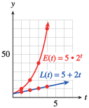
It may be helpful to compare linear growth and exponential growth. Consider the two functions

\begin{equation*} L(t) = 5 + 2t ~\text{ and } ~ E(t) = 5 \cdot 2^t ~~~ (t \ge 0) \end{equation*}

whose graphs are shown in Figure 3.9.

$t$	$L(t)$
$0$	$5$
$1$	$7$
$2$	$9$
$3$	$11$
$4$	$13$

Table 3.7. $m=2$

$t$	$E(t)$
$0$	$5$
$1$	$10$
$2$	$20$
$3$	$40$
$4$	$80$

Table 3.8. Growth factor $b=2$

$L$ is a linear function with initial value $5$ and slope $2\text{;}$ $E$ is an exponential function with initial value $5$ and growth factor $2\text{.}$ In a way, the growth factor of an exponential function is analogous to the slope of a linear function: Each measures how quickly the function is increasing (or decreasing).

However, for each unit increase in $t\text{,}$ $2$ units are added to the value of $L(t)\text{,}$ whereas the value of $E(t)$ is multiplied by $2\text{.}$ An exponential function with growth factor $2$ eventually grows much more rapidly than a linear function with slope $2\text{,}$ as you can see by comparing the graphs in Figure 3.9 or the function values in Tables 3.7 and 3.8.

Example 3.10.

A solar energy company sold $$80,000$ worth of solar collectors last year, its first year of operation. This year its sales rose to $$88,000\text{,}$ an increase of $10$%. The marketing department must estimate its projected sales for the next $3$ years.

If the marketing department predicts that sales will grow linearly, what should it expect the sales total to be next year? Graph the projected sales figures over the next $3$ years, assuming that sales will grow linearly.
If the marketing department predicts that sales will grow exponentially, what should it expect the sales total to be next year? Graph the projected sales figures over the next $3$ years, assuming that sales will grow exponentially.

Solution.

Let $L(t)$ represent the company’s total sales $t$ years after starting business, where $t = 0$ is the first year of operation. If sales grow linearly, then $L(t)$ has the form $L(t) = mt + b\text{.}$ Now $L(0) = 80,000\text{,}$ so the intercept is $(0,80000)\text{.}$ The slope of the graph is

\begin{equation*} \frac{\Delta S}{\Delta t}= \frac{8000 \text{ dollars}}{1\text{ year}}= 8000 \text{ dollars/year} \end{equation*}

where $\Delta S = 8000$ is the increase in sales during the first year. Thus, $L(t) = 8000t + 80,000\text{,}$ and sales grow by adding $$8000$ each year. The expected sales total for the next year is

\begin{equation*} L(2) = 8000(2) + 80,000 = 96,000. \end{equation*}

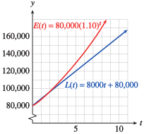
The values of $L(t)$ for $t=0$ to $t=4$ are shown in the middle column of Table 3.11. The linear graph of $L(t)$ is shown in Figure 3.12.
Let $E(t)$ represent the company’s sales assuming that sales will grow exponentially. Then $E(t)$ has the form $E(t) = E_0b^t$ . The percent increase in sales over the first year was $r = 0.10\text{,}$ so the growth factor is

\begin{equation*} b = 1 + r = 1.10 \end{equation*}

The initial value, $E_0\text{,}$ is $80,000\text{.}$ Thus, $E(t) = 80,000(1.10)^t\text{,}$ and sales grow by being multiplied each year by $1.10\text{.}$ The expected sales total for the next year is

\begin{equation*} E(2) = 80,000(1.10)^2= 96,800. \end{equation*}

The values of $E(t)$ for $t=0$ to $t=4$ are shown in the last column of Table 3.11. The exponential graph of $E(t)$ is shown in Figure 3.12.

$t$ $L(t)$ $E(t)$

$0$ $80,000$ $80,000$

$1$ $88,000$ $88,000$

$2$ $96,000$ $96,800$

$3$ $104,000$ $106,480$

$4$ $112,000$ $117,128$

Table 3.11.

linear and exponential growth

Figure 3.12.

Example 3.13.

A new car begins to depreciate in value as soon as you drive it off the lot. Some models depreciate linearly, and others depreciate exponentially. Suppose you buy a new car for $$20,000\text{,}$ and $1$ year later its value has decreased to $$17,000\text{.}$

If the value decreased linearly, what was its annual rate of decrease?
If the value decreased exponentially, what was its annual decay factor? What was its annual percent depreciation?
Calculate the value of your car when it is $5$ years old under each assumption, linear or exponential depreciation.

Solution.

If the annual rate of decrease is $m\text{,}$ then

\begin{equation*} 20000-m=17000\text{.} \end{equation*}

Thus $m=3000$ so the rate of decrease is $\$3000$ per year
If the annual decay factor is $b\text{,}$ then

\begin{equation*} 20000b=17000 \end{equation*}

Thus $b= 0.85$ so the annual decay factor is $0.85\text{.}$ The annual percent depreciation is the percent change from $\$20,000$ to $\$17,000\text{:}$

\begin{equation*} \text{percent change}=\frac{\text{amount change}}{\text{original amount}}=\frac{\$17,000-\$20,000}{\$20,000}=-0.15 \end{equation*}

Therefore the car’s value depreciated by $15\%\text{.}$
Based on the work above, if the car’s value decreased linearly then the value of the car after $t$ years is

\begin{equation*} L(t)=20000-3000t \end{equation*}

If the value of the car depreciated exponentially, then the value of the car after $t$ years is

\begin{equation*} E(t)=20000\cdot0.85^t \end{equation*}

After $5$ years,

\begin{equation*} \begin{aligned} L(5)\amp=20000-3000(5)=5000 \\ E(5)\amp=20000\cdot0.85^5\approx8874 \end{aligned} \end{equation*}

After $5$ years, the car will be worth $\$5000$ under the linear model and worth approximately $\$8874$ under the exponential model.

In the last section, we listed several properties of exponential functions; namely, for $f(x)=a(b)^x$ with $a>0\text{,}$

The domain is all real numbers and the range is all positive numbers.
If $b>1$ then the function is increasing, if $0\lt b\lt 1$ then the function is decreasing.
The $y$-intercept is $(0,a)\text{;}$ there is no $x$-\intercept.

Not convinced of the Properties of Exponential Functions listed above? Try varying the $a$ and $b$ parameters in the following applet to see many more examples of graphs of exponential functions, and convince yourself that the properties listed above hold true.

Figure 3.14. Explore the inverse relationship between between the functions $f(t)=\log_b(t)$ and $g(t)=b^t$ for various values of $b>0$ with this applet.

Exercises 3.2.4 Exercises

1. Properties of Exponential Functions.

a) Suppose we have $f\left(t\right) = 7\left(1.41\right)^{t}\text{.}$ What is the initial value of the function? What is the growth rate? What is the growth factor?

Initial value:

Growth rate:

Growth factor:

b) Suppose we have $f\left(t\right) = 5\left(0.19\right)^{t}\text{.}$ What is the initial value of the function? What is the growth rate? What is the growth factor?

Initial value:

Growth rate:

Growth factor:

Hint.

Recall the exponential formula

\begin{equation*} y=a(b)^t, \end{equation*}

where $a$ is the initial value and $b$ is the growth factor. We have that $b=1+r\text{,}$ where $r$ is the growth factor. To find $r\text{,}$ you want to solve the last equation for $r\text{.}$

2. Comparing Exponential Functions.

Your boss proposes two different plans for giving raises. Suppose you currently earn 75000 dollars per year. In Plan 1, you earn an additional 1500 dollars each year. In Plan 2, you increase your salary by 3 percent each year. Which plan do you think is better? Check your guess by computing your annual salary after 5 years and after 10 years under both plans.

Plan 1:

After 5 years:

After 10 years:

Plan 2:

After 5 years:

After 10 years:

Hint.

Plan 1 is linear growth, so it will be of the form $A(t) = b+mt\text{,}$ where $b$ is the initial amount and $m$ is the constant additional amount of money you earn each year.

Plan 2 is exponential growth, so it will be of the form $P(t)=a(b)^t\text{,}$ where $a$ is the initial amount and $b=1+r$ with growth rate $r\text{.}$

3. Writing Exponential Functions.

Suppose a city has a population of 400,000 at time $t=0\text{,}$ where $t$ is the number of years since 1990.

a) If the city’s population decreases by 4000 people per year, find a formula for $P_1(t)\text{,}$ the city’s population $t$ years after 1990.

$P_1(t) =$

b) If the city’s population decreases by 7 percent per year, find a formula for $P_2(t)\text{,}$ the city’s population $t$ years after 1990.

$P_2 (t) =$

Hint.

a) In this part, the population is decreasing by a constant value per year, from which we know this is a linear equation. Recall a linear function is of the form

\begin{equation*} y=mt+b, \end{equation*}

where $b$ is the initial value and $m$ is the constant rate of change.

b) Here, the population is decreasing by a certain percentage each year, which indicates this will be best represented by an exponential function. Recall an exponential function is of the form

\begin{equation*} y=a(b)^t, \end{equation*}

where $a$ is the initial value and $b$ is the growth factor (we know $b=1+r\text{,}$ where $r$ is the growth rate).

4. Linear vs. Exponential Functions: Tables.

Decide whether each of $h(x)$ and $k(x)$ could be a linear or exponential function. Then, find a possible formula for the function.

$x$	$0$	$1$	$2$	$3$	$4$
$h(x)$	$6$	$5.1$	$4.2$	$3.3$	$2.4$

Values of $h(x)$

Linear
Exponential

Formula for $h(x)\text{:}$

$x$	$0$	$2$	$3$	$5$	$6$
$k(x)$	$3$	$12$	$24$	$96$	$192$

Values of $k(x)$

Linear
Exponential

Formula for $k(x)\text{:}$

Hint.

For each of these tables you should determine you add a constant for each increase by 1 in $x$ or if you multiply by a constant for each increase by 1 in $x\text{.}$

A linear function can be verified by checking that there’s a constant average rate of change in the table:

\begin{equation*} \frac{f(b)-f(a)}{b-a}. \end{equation*}

An exponential function can be verified by checking that there’s a constant ratio between values in the table.

Recall the formulas for a linear and an exponential function:

\begin{equation*} \text{Linear: } y=mt+b \end{equation*}

\begin{equation*} \text{Exponential: } y=a(b)^t. \end{equation*}

Note the "b"s in each equation represent different values!

5. Linear vs. Exponential Functions: Writing Formulas.

In 1987, there were 7,261,711 Americans who held valid US passports. It is also known that 131,841,062 Americans held valid US passports in 2015. Write a formula for the number of Americans with valid US passports $t$ years after 1987 if the growth of passport holders is...

a) linear

b) exponential

Hint.

Recall the formulas for a linear function and an exponential function:

\begin{equation*} \text{Linear: } y=mt+b, \end{equation*}

where $m$ is the constant average rate of change and $b$ is the initial value, and

\begin{equation*} \text{Exponential: } y=a(b)^t, \end{equation*}

where $a$ is the initial value and $b$ is the growth factor.

a) Recall the slope formula:

\begin{equation*} m=\frac{y_2=y_1}{t_2-t_1}. \end{equation*}

Use the given information to calculate the slope for the equation.

b) Recall that an exponential function has a constant factor $b$ which we multiply each time we increase $t$ by 1. Starting in 1987, there were 7,261,711 Americans with valid US passports. To get to the year 2015, think about how many times you would need to multiply by your growth factor $b\text{.}$ Set up an equation relating $b\text{,}$ 7,261,711, and 131,841,062 based on the information given. You’ll use this to solve for $b\text{.}$

6. Linear vs. Exponential Functions: Tables.

The approximate GDPs per capita of two countries from 2000 to 2004 (in today’s US dollars) are shown in the table below. For each country, determine whether the GDP per capita is better modeled by a linear or exponential function, and write a formula modeling the GDP per capita as a function of years since 2000.

Years since 2000	$0$	$1$	$2$	$3$	$4$
GDP per capita	$35,400$	$36,900$	$38,400$	$39,900$	$41,400$

Country A

Years since 2000	$0$	$1$	$2$	$3$	$4$
GDP per capita	$23,700$	$25,738$	$27,952$	$30,356$	$32,966$

Country B

Country A:

Linear
Exponential

$A(t)=$

Country B

Linear
Exponential

$B(t) =$

Hint.

For each of these tables you should determine you add a constant for each increase by 1 in $x$ or if you multiply by a constant for each increase by 1 in $x\text{.}$

A linear function can be verified by checking that there’s a constant average rate of change in the table:

\begin{equation*} \frac{f(b)-f(a)}{b-a}. \end{equation*}

An exponential function can be verified by checking that there’s a constant ratio between values in the table.

Recall the formulas for a linear and an exponential function:

\begin{equation*} \text{Linear: } y=mt+b \end{equation*}

\begin{equation*} \text{Exponential: } y=a(b)^t. \end{equation*}

Note the "b"s in each equation represent different values!

7. Linear vs. Exponential Functions: Writing Formulas.

An ornithologist decides to track the population of American goldfinches in her neighborhood. In 2011, she observes that there are 4 goldfinches in her neighborhood. In 2018, she records that there are 16 goldfinches. Let $P(t)$ be the number of goldfinches in the neighborhood $t$ years after 2011.

a) Assuming the goldfinch population is growing linearly, find a formula for $P(t)\text{.}$

$P(t) =$

Interpret the slope $m$ of $P(t)$ in the context of the problem.

The ornithologist sees $m$ goldfinches every day.
For every increase by 1 goldfinch, $m$ years have passed.
$m$ goldfinches leave the neighborhood every year.
Each year, the goldfinch population increases by $m$ birds.

b) Assuming the goldfinch population is growing exponentially, find a formula for $P(t)\text{.}$

$P(t) =$

Interpret the growth rate $g$ of $P(t)$ in the context of the problem.

Every year, the goldfinch population grows by about $g$ percent.
Every day, the ornithologist feeds $g$ percent of the goldfinches.
The goldfinch population grows by about $g$ goldfinches each year.
After about $g$ years, the goldfinch population will increase by 12.

Hint.

For both parts, $P(0) =4$ and $P(7) = 9\text{.}$

a) Recall the formula for a linear function

\begin{equation*} y=mt+b, \end{equation*}

where $m$ is the slope and $b$ is the initial value. Recall the slope formula:

\begin{equation*} m=\frac{y_2-y_1}{x_2-x_1}. \end{equation*}

For the interpretation, remember that $m$ is a rate of change.

b) Recall the formula for an exponential function

\begin{equation*} y=a(b)^t, \end{equation*}

where $a$ is the initial value and $b$ is the growth factor. For the interpretation, remember that $g$ (the growth rate) is often represented as a percentage.

8. Exponential Functions: Graph.

a) Assuming the goldfinch population is growing linearly, find a formula for $P(t)\text{.}$

$P(t) =$

Interpret the slope $m$ of $P(t)$ in the context of the problem.

For every increase by 1 goldfinch, $m$ years have passed.
$m$ goldfinches leave the neighborhood every year.
Each year, the goldfinch population increases by $m$ birds.
The ornithologist sees $m$ goldfinches every day.

b) Assuming the goldfinch population is growing exponentially, find a formula for $P(t)\text{.}$

$P(t) =$

Interpret the growth rate $g$ of $P(t)$ in the context of the problem.

Every year, the goldfinch population grows by about $g$ percent.
Every day, the ornithologist feeds $g$ percent of the goldfinches.
The goldfinch population grows by about $g$ goldfinches each year.
After about $g$ years, the goldfinch population will increase by 12.

Hint.

For both parts, $P(0) =4$ and $P(7) = 9\text{.}$

a) Recall the formula for a linear function

\begin{equation*} y=mt+b, \end{equation*}

where $m$ is the slope and $b$ is the initial value. Recall the slope formula:

\begin{equation*} m=\frac{y_2-y_1}{x_2-x_1}. \end{equation*}

For the interpretation, remember that $m$ is a rate of change.

b) Recall the formula for an exponential function

\begin{equation*} y=a(b)^t, \end{equation*}

where $a$ is the initial value and $b$ is the growth factor. For the interpretation, remember that $g$ (the growth rate) is often represented as a percentage.

9. Computing Exponential Growth.

The processing power of a computer is essentially how quickly the computer can perform tasks and calculations. The higher the number of transistors in an integrated circuit, the more processing power that computer has. In 1975, Gordon Moore predicted that the number of transistors in a dense integrated circuit doubles every two years. So far, the so-called ``Moore’s Law" has proven to be accurate.

a) If there were 2574 transistors in an integrated circuit in 1971, write a formula for the number of transistors as a function of $t$ years since 1971.

b) About how much (as a percentage) does computing power increase each year?

percent

Hint.

a) We are looking for a formula of the form $A(t) = a(b)^t\text{,}$ where $a$ is the initial value and $b$ is the growth factor. Think about what the information that the number of transistors doubles every two years tells you in this case. It may be helpful to set up the following formula:

\begin{equation*} 2a=a(b)^2, \end{equation*}

since the initial value $a$ will double when $t=2\text{.}$ Use this information to find $b\text{.}$

b) Here we want to know the growth rate, which will be given by taking $b-1\text{.}$ Make sure to convert this to a percentage.

Prev Top Next

\(t\)	\(L(t)\)
\(0\)	\(5\)
\(1\)	\(7\)
\(2\)	\(9\)
\(3\)	\(11\)
\(4\)	\(13\)

\(t\)	\(E(t)\)
\(0\)	\(5\)
\(1\)	\(10\)
\(2\)	\(20\)
\(3\)	\(40\)
\(4\)	\(80\)

\(t\)	\(L(t)\)	\(E(t)\)
\(0\)	\(80,000\)	\(80,000\)
\(1\)	\(88,000\)	\(88,000\)
\(2\)	\(96,000\)	\(96,800\)
\(3\)	\(104,000\)	\(106,480\)
\(4\)	\(112,000\)	\(117,128\)