- A Hamiltonian circuit is a circuit that visits every vertex once with no repeats. Being a circuit, it must start and end at the same vertex.
- A Hamiltonian path also visits every vertex once with no repeats, but does not have to start and end at the same vertex.
Section 16.1 Hamilton Circuits and the Traveling Salesperson Problem
In the last section, we considered optimizing a walking route for a postal carrier. How is this different than the requirements of a package delivery driver? While the postal carrier needed to walk down every street (edge) to deliver the mail, the package delivery driver instead needs to visit every one of a set of delivery locations. Instead of looking for a circuit that covers every edge once, the package deliverer is interested in a circuit that visits every vertex once.
Hamiltonian paths and circuits are named for William Rowan Hamilton who studied them in the 1800’s. Sometimes you will see them referred to simply as Hamilton paths and circuits.
Example 16.1.1.
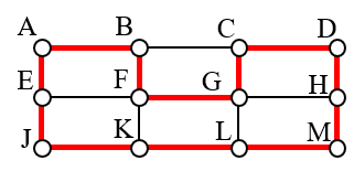
One Hamiltonian circuit is shown on the graph below. There are several other Hamiltonian circuits possible on this graph. Notice that the circuit only has to visit every vertex once; it does not need to use every edge.
This circuit could be notated by the sequence of vertices visited, starting and ending at the same vertex: ABFGCDHMLKJEA. Notice that the same circuit could be written in reverse order, or starting and ending at a different vertex.
Unlike with Euler circuits, there is no nice theorem that allows us to instantly determine whether or not a Hamiltonian circuit exists for all graphs.
1
There are some theorems that can be used in specific circumstances, such as Dirac’s theorem, which says that a Hamiltonian circuit must exist on a graph with \(n\) vertices if each vertex has degree \(n/2\) or greater.
Example 16.1.2.
Does a Hamiltonian path or circuit exist on the graph below?
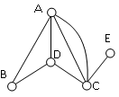
We can see that once we travel to vertex E there is no way to leave without returning to C, so there is no possibility of a Hamiltonian circuit. If we start at vertex E we can find several Hamiltonian paths, such as ECDAB and ECABD.
With Hamiltonian circuits, our focus will not be on existence, but on the question of optimization; given a graph where the edges have weights, can we find the optimal Hamiltonian circuit; the one with lowest total weight.
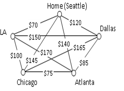
This problem is called the Traveling Salesperson Problem (TSP) because the question can be framed like this: Suppose a salesperson needs to give sales pitches in five cities. He looks up the airfares between each city, and puts the costs in a graph. In what order should he travel to visit each city once then return home with the lowest cost? A situation like this could be represented with the graph shown at right.
To answer this question of how to find the lowest cost Hamiltonian circuit, we will consider some possible approaches. The first option that might come to mind is to just try all different possible circuits.
Brute Force Algorithm (exhaustive search).
- List all possible Hamiltonian circuits.
- Find the length of each circuit by adding the edge weights.
- Select the circuit with minimal total weight.
Example 16.1.3.
Apply the Brute Force Algorithm to find the minimum cost Hamiltonian circuit on the graph below.
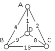
To apply the Brute Force Algorithm, we list all possible Hamiltonian circuits and calculate their weight:
| Circuit | Weight |
| ABCDA | \(4+13+8+1 = 26\) |
| ABDCA | \(4+9+8+2 = 23\) |
| ACBDA | \(2+13+9+1 = 25\) |
Note: These are the unique circuits on this graph. All other possible circuits are the reverse of the listed ones or start at a different vertex, but result in the same weights. For example, the circuits ABCDA, BCDAB, BADCB, and DABCD are all the same, so we only list one of them on the table.
From this we can see that the second circuit, ABDCA, is the optimal circuit.
The Brute Force Algorithm is optimal; it will always produce the Hamiltonian circuit with minimum weight. Is it efficient? To answer that question, we need to consider how many Hamiltonian circuits a graph could have. For simplicity, let’s look at the worst-case possibility, where every vertex is connected to every other vertex. This is called a complete graph.
Using a type of mathematics called combinatorics, we can find a formula that gives the number of unique Hamilton circuits for a complete graph with any number, \(n\text{,}\) of vertices. The results are as follows:
| Number of vertices | Number of unique Hamilton circuits |
| \(4\) | \(3\) |
| \(5\) | \(12\) |
| \(6\) | \(60\) |
| \(7\) | \(360\) |
| \(8\) | \(2520\) |
| \(9\) | \(20,160\) |
| \(10\) | \(181,440\) |
| \(15\) | \(43,589,145,600\) |
| \(20\) | \(60,822,550,204,416,000\) |
As you can see, the number of circuits starts small but grows extremely quickly. If a computer looked at one billion circuits a second, it would still take almost two years to examine all the possible circuits with only 20 vertices. With 30 vertices, the most powerful supercomputer in the world would take about 140 million years to do so! Certainly Brute Force is not an efficient algorithm.
Unfortunately, no one has yet found an efficient and optimal algorithm to solve the TSP, and it is very unlikely anyone ever will. Since it is not practical to use Brute Force to solve the problem, we turn instead to heuristic algorithms: efficient algorithms that give approximate solutions. In other words, heuristic algorithms are fast, but are not guaranteed to produce the optimal circuit.
2
This is actually related to a famous problem in computer science. It is considered important enough that a $1 million reward has been offered for a solution.
Nearest Neighbor Algorithm (NNA).
- Select a starting point.
- Move to the nearest unvisited vertex (the edge with smallest weight).
- Repeat until the circuit is complete.
Example 16.1.6.
Consider our earlier graph (from Example 16.1.3), shown below.
- Starting at vertex A, the nearest neighbor is vertex D with a weight of 1.
- From D, the nearest neighbor is C, with a weight of 8.
- From C, our only option is to move to vertex B, the only unvisited vertex, with a cost of 13.
- From B we return to A with a weight of 4.
The resulting circuit is ADCBA with a total weight of \(1+8+13+4 = 26\text{.}\)
We ended up finding the worst circuit in the graph! What happened? Unfortunately, while it is very easy to implement, the NNA is a greedy algorithm, meaning it only looks at the immediate decision without considering the consequences in the future. In this case, following the edge AD forced us to use the very expensive edge BC later.
Example 16.1.7.
Consider again a salesperson visiting the five cities shown in the graph below. Starting in Seattle, the nearest neighbor (cheapest flight) is to LA, at a cost of $70. From there:
- LA to Chicago: $100
- Chicago to Atlanta: $75
- Atlanta to Dallas: $85
- Dallas to Seattle: $120
- Total cost: $450
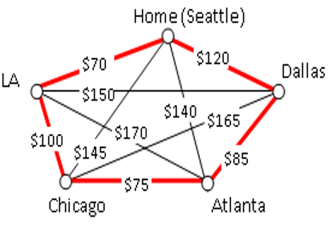
In this case, nearest neighbor did find the optimal circuit.
Going back to Example 16.1.6, how could we improve the outcome? One option would be to redo the nearest neighbor algorithm with a different starting point to see if the result changed. Since nearest neighbor is so fast, doing it several times isn’t a big deal.
Repeated Nearest Neighbor Algorithm (RNNA).
- Do the Nearest Neighbor Algorithm starting at each vertex.
- Choose the circuit produced with minimal total weight.
Example 16.1.8.
We will revisit the graph from Example 16.1.6.
- Starting at vertex A resulted in a circuit with weight 26.
- Starting at vertex B, the nearest neighbor circuit is BADCB with a weight of \(4+1+8+13 = 26\text{.}\) This is the same circuit we found starting at vertex A. No better.
- Starting at vertex C, the nearest neighbor circuit is CADBC with a weight of \(2+1+9+13 = 25\text{.}\) Better!
- Starting at vertex D, the nearest neighbor circuit is DACBA. Notice that this is actually the same circuit we found starting at C, just written with a different starting vertex.
The RNNA was able to produce a slightly better circuit with a weight of 25, but still not the optimal circuit in this case. Notice that even though we found the circuit by starting at vertex C, we could still write the circuit starting at A: ADBCA or ACBDA.
Exploration 16.1.1.
The table below shows the time, in milliseconds, it takes to send a packet of data between computers on a network. If data needed to be sent in sequence to each computer, then notification needed to come back to the original computer, we would be solving the TSP. The computers are labeled A-F for convenience.
| A | B | C | D | E | F | |
| A | -- | 44 | 34 | 12 | 40 | 41 |
| B | 44 | -- | 31 | 43 | 24 | 50 |
| C | 34 | 31 | -- | 20 | 39 | 27 |
| D | 12 | 43 | 20 | -- | 11 | 17 |
| E | 40 | 24 | 39 | 11 | -- | 42 |
| F | 41 | 50 | 27 | 17 | 42 | -- |
- Find the circuit generated by the NNA starting at vertex B.
- Find the circuit generated by the RNNA.
Solution.
- At each step, we look for the nearest location we haven’t already visited.
- From B, the nearest computer is E with time 24.
- From E, the nearest computer is D with time 11.
- From D, the nearest is A with time 12.
- From C, the only computer we haven’t visited is F with time 27.
- From F, we return back to B with time 50.
The NNA circuit from B is BEDACFB with time 158 milliseconds. - Using NNA again from other starting vertices:
- Starting at A: ADEBCFA: time 146
- Starting at C: CDEBAFC: time 167
- Starting at E: EDACFBE: time 158
- Starting at D: DEBCFAD: time 146
- Starting at F: FDEBCAF: time 158
The RNNA found a circuit with time 146 milliseconds: ADEBCFA. We could also write this same circuit starting at B if we wanted: BCFADEB or BEDAFCB.
