CM Linear Growth

Section11.1Linear Growth

SubsectionLinear Growth

Marco is a collector of antique soda bottles. His collection currently contains 437 bottles. Every year, he budgets enough money to buy 32 new bottles. Can we determine how many bottles he will have in 5 years, or 20 years? What about how long it will take for his collection to reach 1500 bottles?

To answer the first question, you would probably just add 32 on to his original amount 5 times, like this:

\begin{equation*} \text{After 1 year: } 437 + 32 = 469 \end{equation*}

\begin{equation*} \text{After 2 years: } 469 + 32 = 501 \end{equation*}

\begin{equation*} \text{After 3 years: } 501 + 32 = 533 \end{equation*}

\begin{equation*} \text{After 4 years: } 533 + 32 = 565 \end{equation*}

\begin{equation*} \text{After 5 years: } 565 + 32 = 597 \end{equation*}

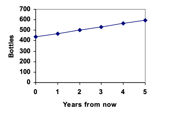
So Marco should have 597 bottles after 5 years. Notice that we can keep adding 32 to get a list of numbers that represent the size of Marco's collection over time. We call such a list of numbers a sequence, and each number in the list a term. However, this repeated addition gets tedious rather quickly, so we should probably find a faster way to calculate the number of bottles after 20 years or more.

As you might have already noticed, we can replace this repeated addition with multiplication:

\begin{equation*} 437 + 32 + 32 + 32 + 32 + 32 = 437 + 5 \times 32 \end{equation*}

We have simply multiplied the number of years (5) by the number of bottles per year (32) to find the total increase in bottles over 5 years, and added it on to his original amount of bottles (437). We can find the size of Marco's collection after 20 years in the same way:

\begin{equation*} 437 + 20 \times 32 = 437 + 640 = 1077 \end{equation*}

This method is much faster, and makes calculating the size of Marco's collection after any number of years manageable.

How can we find how many years it will take for Marco to collect 1500 bottles? One way would be to use guess-and-check. Perhaps we would take a wild guess that it will take around 30 years for him to collect so many, then calculate how many bottles he would actually have collected after 30 years using our method above. Depending on how this calculation compares to 1500, we could then adjust our guess of 30 up or down, and repeat this process until we get close enough to the right number.

However, we can be quicker and more precise about this if we formalize our method above and use it to write an equation relating the number of bottles ($B$) in Marco's collection to the number of years ($n$) it has been:

\begin{equation*} B = 437 + n \times 32 \end{equation*}

(Typically, we would write this as $B = 437 + 32n\text{.}$ This is just a convention.)

Now we can find the number of years it will take to collect 1500 bottles by plugging 1500 in for the number of bottles in this formula, and solving for $n\text{,}$ the number of years:

\begin{equation*} 1500 = 437 + 32n \end{equation*}

\begin{equation*} 1163 = 32n \end{equation*}

\begin{equation*} n = \frac{1163}{32} = 36.34 \end{equation*}

So Marco will reach 1500 bottles during the 37th year.

In this example, Marco's collection grew by the same number of bottles every year. This constant change is the defining characteristic of a linear sequence. Plotting the values we calculated for Marco's collection, we can see the values form a straight line, the shape of a linear sequence.

Linear Sequences

A sequence is linear (or arithmetic) if the difference from one term to the next is always the same.

The difference between any two consecutive terms is called the common difference and is often represented by the letter $d\text{.}$ In the example of Marco's collection, $d = 32\text{.}$

If $d$ is positive, the sequence is increasing, and we say that it exhibits linear growth. If $d$ is negative, the sequence is decreasing.

If a quantity starts at size $P_0$ and grows by $d$ every time period, then the quantity $P$ after $n$ time periods can be determined using this formula:

$\hspace{2.5in} P = P_0 + dn$

You may recognize the common difference, $d\text{,}$ in our linear equation as slope. In fact, the entire explicit equation should look familiar it is the same linear equation you learned in algebra, probably stated as $y = mx + b.$

In the standard algebraic equation $y = mx + b\text{,}$ $b$ was the y-intercept, or the y value when x was zero. In the form of the equation we're using, $P_0$ to represents that initial amount.

In the $y = mx + b$ equation, recall that $m$ was the slope. You might remember this as rise over run, or the change in y divided by the change in x. Either way, it represents the same thing as the common difference, $d\text{,}$ we are using the amount the output $P$ changes when the input n increases by 1.

The equations$y = mx + b$ and $P = P_0 + d n$ mean the same thing and can be used in the same ways; we're just writing it somewhat differently.

Example11.1

The population of elk in a national forest was measured to be 12,000 in 2003, and was measured again to be 15,000 in 2007. If the population continues to grow linearly at this rate, what will the elk population be in 2014?

To begin, we need to define how we're going to measure $n\text{.}$ Remember that $P_0$ is the initial population, when $n = 0\text{,}$ so we probably don't want to literally use the year 0. Since we already know the population in 2003, let us define $n = 0$ to be the year 2003. Then $P_0 = 12,000\text{.}$

Next we need to find $d\text{.}$ Remember $d$ is the growth per time period, in this case growth per year. Between the two measurements, the population grew by $15,000-12,000 = 3,000\text{,}$ but it took $2007-2003 = 4$ years to grow that much. To find the growth per year, we can divide: $\frac{3000 \text{ elk}}{4 \text{ years}} = 750 \text{ elk}$ in 1 year.

Alternatively, you can use the slope formula from algebra to determine the common difference, noting that the population is the output of the formula, and time is the input.

\begin{equation*} d = slope = \frac{\text{change in output}}{\text{change in input}} = \frac{15,000-12,000}{2007-2003} = \frac{3000}{4} = 750 \end{equation*}

We can now write an equation for the growth of the elk population:

\begin{equation*} P = 12,000 + 750n \end{equation*}

To answer the question, we need to first note that the year 2014 will be $n = 11\text{,}$ since 2014 is 11 years after 2003. Let's use our equation for this calculation:

\begin{equation*} 12,000 + 750(11) = 20,250 \text{ elk} \end{equation*}

Example11.2

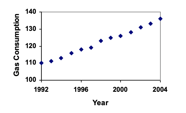
Gasoline consumption in the US has been increasing steadily. Consumption data from 1992 to 2004 is shown below¹http://www.bts.gov/publications/national_transportation_statistics/2005/html/table_04_10.html in billions of gallons. Find a model for this data, and use it to predict consumption in 2016. If the trend continues, when will consumption reach 200 billion gallons?

Year	'92	'93	'94	'95	'96	'97	'98	'99	'00	'01	'02	'03	'04
Consumption (bil. gal)	110	111	113	116	118	119	123	125	126	128	131	133	136

Plotting this data, it appears to have an approximately linear relationship: While there are more advanced statistical techniques that can be used to find an equation to model the data, to get an idea of what is happening, we can find an equation by using two pieces of the data perhaps the data from 1993 and 2003.

Letting $n=0$ correspond with 1993 would give $P_0 = 111$ billion gallons.

To find $d\text{,}$ we need to know how much the gas consumption increased each year, on average. From 1993 to 2003 the gas consumption increased from 111 billion gallons to 133 billion gallons, a total change of $133 111 = 22$ billion gallons, over 10 years. This gives us an average change of $\frac{22 \text{ billion gallons}}{10 \text{ years}} = 2.2$ billion gallons per year.

Equivalently,

\begin{equation*} d = slope = \frac{\text{change in output}}{\text{change in input}} = \frac{113-111}{10-0} = \frac{22}{10} = 2.2 \text{ billion gallons per year} \end{equation*}

We can now write an equation for the growth of gas consumption, in billions of gallons:

\begin{equation*} P = 111 + 2.2n \end{equation*}

Calculating values using this formula and plotting them with the original data shows how well our model fits the data.

We can now use our model to make predictions about the future, assuming that the previous trend continues unchanged. To predict the gasoline consumption in 2016:

$n = 23$ (2016-1993 = 23 years later)

$111 + 2.2(23) = 161.6$

Our model predicts that the US will consume 161.6 billion gallons of gasoline in 2016 if the current trend continues.

To find when the consumption will reach 200 billion gallons, we would set $P = 200\text{,}$ and solve for $n\text{:}$

$P = 200$	Replace $P$ with our model
$111 + 2.2n = 200$	Subtract 111 from both sides
$2.2n = 89$	Divide both sides by 2.2
$n=40.4545$

Example11.3

The cost, in dollars, of a gym membership for n months can be described by the equation $P = 70 + 30n\text{.}$ What does this equation tell us?

The value for $P_0$ in this equation is 70, so the initial starting cost is $70. This tells us that there must be an initiation or start-up fee of $70 to join the gym.

The value for $d$ in the equation is 30, so the cost increases by $30 each month. This tells us that the monthly membership fee for the gym is $30 a month.

Exploration11.1

The number of stay-at-home fathers in Canada has been growing steadily ²http://www.fira.ca/article.php?id=140. While the trend is not perfectly linear, it is fairly linear. Use the data from 1976 and 2010 to find a formula for the number of stay-at-home fathers, then use it to predict the number in 2020.

Year	1976	1984	1991	2000	2010
# Stay at home fathers	20,610	28,725	43,530	47,664	53,555

Solution

Letting $n = 0$ correspond with 1976, then $P_0 = 20,610\text{.}$

From 1976 to 2010 the number of stay-at-home fathers increased by $53,555 20,610 = 32,945\text{.}$

This happened over 34 years, giving a common different $d$ of $\frac{32,945}{34} = 969\text{.}$

$P = 20,610 + 969n$

SubsectionWhen good models go bad

When using mathematical models to predict future behavior, it is important to keep in mind that very few trends will continue indefinitely.

Example11.4

Suppose a four year old boy is currently 39 inches tall, and you are told to expect him to grow 2.5 inches a year.

We can set up a growth model, with $n = 0$ corresponding to 4 years old.

\begin{equation*} P = 39 + 2.5n \end{equation*}

So at 6 years old, $n = 2\text{,}$ and we expect him to be:

$39+2.5(2) = 44$ inches tall.

Any mathematical model will break down eventually. Certainly, we shouldn't expect this boy to continue to grow at the same rate all his life. If he did, at age 50 he would be $39 + 2.5(46) = 154$ inches tall = 12.8 feet tall!

When using any mathematical model, we have to consider which inputs are reasonable to use. Whenever we extrapolate, or make predictions into the future, we are assuming the model will continue to be valid.

\(P = 200\)	Replace \(P\) with our model
\(111 + 2.2n = 200\)	Subtract 111 from both sides
\(2.2n = 89\)	Divide both sides by 2.2
\(n=40.4545\)