What proportion of adults have systolic blood pressure above 140? What is the probability of getting more than 250 heads in 400 tosses of a fair coin? If the average weight of a piece of carry-on luggage is 11 pounds, what is the probability that 200 random carry on pieces will weigh more than 2500 pounds? If 55% of a population supports a certain candidate, what is the probability that she will have less than 50% support in a random sample of size 200?
There is one distribution that can help us answer all of these questions. Can you guess what it is? That’s right – it’s the normal distribution.
Among all the distributions we see in practice, one is overwhelmingly the most common. The symmetric, unimodal, bell curve is ubiquitous throughout statistics. Indeed it is so common, that people often know it as the normal curve or normal distribution.
Normal distribution.
We say that data is normally distributed when the corresponding histogram is bell-shaped.
The normal distribution always describes a symmetric, unimodal, bell-shaped curve. However, these curves can look different depending on the details of the model.
The x-value of the center of the bell corresponds to the population mean, which we will denote by the greek symbol \(\mu \text{,}\) pronounced "m-yoo". The standard deviation \(\sigma\) is the distance from the mean to a point about halfway up a curve. It tells us how spread apart the data is.
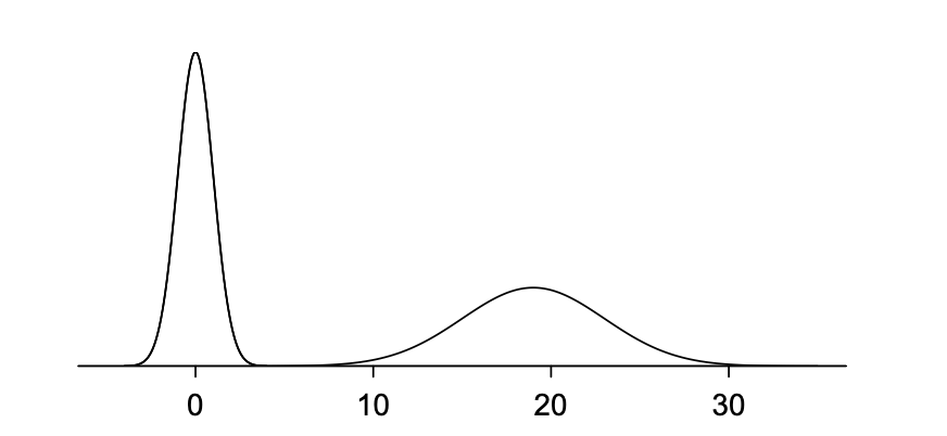
Th normal distribution model can be adjusted using these two parameters. As you can probably guess, changing the mean shifts the bell curve to the left or right, while changing the standard deviation stretches or constricts the curve. Figure 4.1 shows the normal distribution with mean 0 and standard deviation 1 in the left panel and the normal distributions with mean 19 and standard deviation 4 in the right panel. Figure 4.2 shows these distributions on the same axis.
Figure4.1.1.Both curves represent the normal distribution. However, they differ in their center and spread.
Figure4.1.2.The normal distributions shown in Figure 4.1 but plotted together and on the same scale.
As you can see above, a normal distribution with a larger standard deviation will have a wider bell shape than one with a smaller standard deviation.
Subsection4.1.2The 68-95-99.7 Rule
Here, we present a useful rule of thumb for the probability of falling within 1, 2, and 3 standard deviations of the mean in the normal distribution. This will be useful in a wide range of practical settings, especially when trying to make a quick estimate without a calculator.
The 68-95-99.7 Rule.
The 68-95-99.7 rule tells us that in a normal distribution:
Approximately 68% of normally distributed data lies within 1 standard deviation of the mean.
Approximately 95% of normally distributed data lies within 2 standard deviations of the mean.
Approximately 99.7% of normally distributed data lies within 3 standard deviations of the mean.
In terms of probability, this means that there is a 68% probability of an observation falling within 1 standard deviation of the mean. Similarly, there’s a 95% chance or a 99.7% of an observation falling within 2 or 3 standard deviations of the mean respectively.
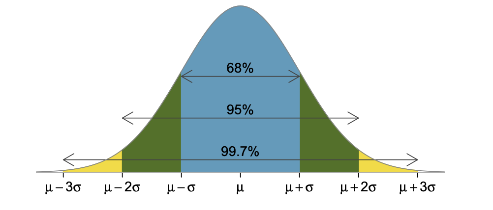
We can see this information represented graphically below:
Figure4.1.3.Probabilities for falling within 1,2, and 3 standard deviations of the mean in a normal distribution.
Example4.1.4.
SAT scores closely follow the normal model with mean \(\mu = 1100 \) and standard deviation \(\sigma = 200\text{.}\)
About what percent of test takers score 700 to 1500?
700 and 1500 represent two standard deviations above and below the mean respectively, which means about 95% of test takers score between 700 and 1500.
What percent score between 1100 and 1500?
Since the normal model is symmetric, half of the test takers from part 1 (95%/2 = 47.5%) will score between 700 and 1100 while the remaining 47.5% will score between 1100 and 1500.
Example4.1.5.
In the example above, we saw that SAT scores follow a normal distribution with a mean of 1100 and a standard deviation of 200.
How high are the top 2.5% of scores?
We know that 95% of SAT scores are within two standard deviations from the mean, so 5% are greater than two standard deviations away. From the symmetry of the normal curve, we know that the top 2.5% of the SAT scores the ones that are more than 2 standard deviations larger than the mean. So the top 2.5% of SAT scores range from 1500 to 1600 (the maximum possible score).
How low are the lowest 16% of scores?
We know that 68% of the SAT scores are within one standard deviation away from the mean. The remaining 32% are more than one standard deviation from the mean. The lowest 16% of scores are those that are more than 2 standard deviations less than the mean. The lowest 16% of scores are all scores less than 1100.
Example4.1.6.
We can also use the normal distribution to discuss probability.
What is the probability that a test taker scores between 900 and 1300 on the SAT? We know that all of the data points between 900 and 1300 make up 68% of the SAT scores, so the probability of a score falling between those two scores is 0.68.