Most of the real-world graphs we’ve seen so far have vertices representing a single type of object, and edges representing a symmetric relationship that the vertices can have with each other. For example, in a graph of people and friendships, the vertices are all people, and each edge represents a friendship, where if Amy is a friend of Tom, then Tom is also a friend of Amy. Or in a graph of the streets in a neighborhood, the vertices are all intersections and the edges are connections between them, where if intersection A is connected to intersection B by a street, then intersection B is connected to intersection A by the same street.
However, there are also many situations where we might want to consider multiple types of objects as vertices, with edges representing asymmetric relationships between two vertices of different types. For example, consider the graph where each vertex is either a house or a person, and two vertices are connected by an edge if one of them is an owner of the other. Amy owns her house, so there is an edge between them, but her house does not own her! This is an example of a bipartite graph.
Bipartite Graphs.
A bipartite graph is a graph in which the vertices can be divided into two parts, with no edges between vertices from the same part.
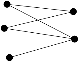
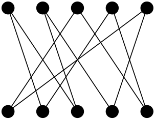
We will often draw bipartite graphs with the two parts being top and bottom, or left and right, as shown here:
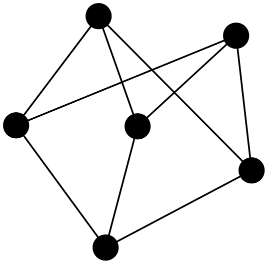
Of course, not all bipartite graphs need to look bipartite, with the different parts grouped in different areas of the drawing. For example, consider this graph:
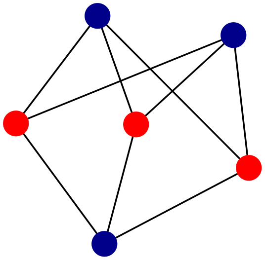
At first glance, it isn’t clear how to group the vertices into two distinct parts, with no edges connecting vertices from the same part. However, if we color the vertices, as below, we can see that no two blue vertices are connected, and no two red vertices are connected. So the blue collection and red collection make up the two parts, demonstrating that this graph is bipartite.
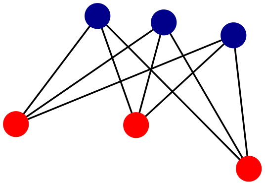
We can also move some of the vertices around to make the two parts more obviously distinct. In this case, just moving the bottom blue vertex up towards the top of the picture makes it look like this:
Subsection17.1.2Matchings
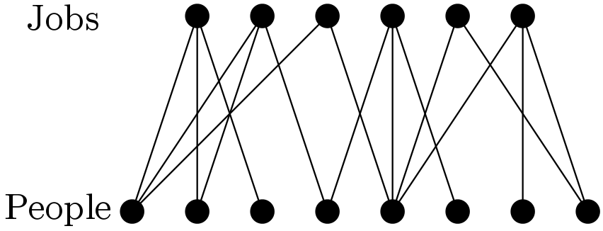
Oftentimes, bipartite graphs are useful to consider because we want to find a way to pair vertices from one part with vertices from another part. For example, we might have a number of job openings, and we want to give each job to a person who is qualified for it. We might consider the bipartite graph where vertices are jobs and people, and an edge connects a job and a person whenever that person is qualified for that job. For example, the graph might look like this:
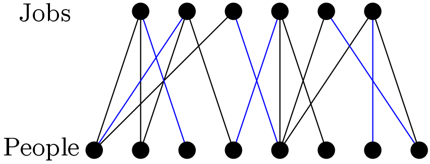
Let’s assume that each person can only work one job, and each job will be given to only one person. Then a way to fill all of the job openings corresponds to a particular collection of edges; each edge pairs one person with one job. For example, we might fill the jobs by picking all of the blue edges below. Each job is given to the person connected to it by a blue edge.
Notice that no vertex is on two different blue edges, since that would either correspond to a job that is given to two different people, or a person who is given two different jobs (both of which we’re assuming shouldn’t happen). A collection of edges that satisfies this property is called a matching.
Matchings.
A matching is a collection of edges where no two edges share a vertex. In other words, a matching is a way of pairing up vertices that are connected.
We will notate matchings by listing their edges. For example, matching vertex A with vertex C and vertex B with vertex D could be notated as {AC, BD}.
A perfect matching is a matching where every vertex in the graph is included in some edge from the matching. A perfect matching is appropriate when we want to find a way to include every vertex in some pair.
Notice that the matching from our example above is not a perfect matching. Although all the jobs are included in some edge of the matching, not all the people are. Unfortunately, a perfect matching in this graph is impossible, because there are more people than jobs.
Example17.1.1.
UNL’s mathematics graduate students engage in a mentorship program, where each incoming graduate student is paired with a more experienced graduate student who acts as their mentor. The pairs are assigned based on shared interest areas, as well as other compatibility factors.
The process of assigning mentors can be thought of as finding a matching in a bipartite graph. There are two groups of vertices: incoming students, and experienced students who are willing to act as mentors. An edge between an incoming student and an experienced student indicates that the pair is compatible. A matching in this graph would represent a way of assigning a mentor to some collection of incoming students. This need not be a perfect matching; there is no need for every experienced student to act as a mentor. However, we do at least want a matching that covers all of the incoming students, so that all of them have mentors.
Exploration17.1.1.
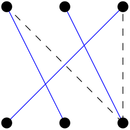
If possible, find a perfect matching for each of the following graphs. If not, find a matching that covers as many vertices as possible.
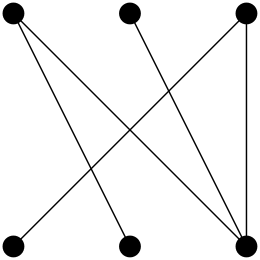
Figure17.1.2.
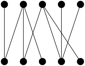
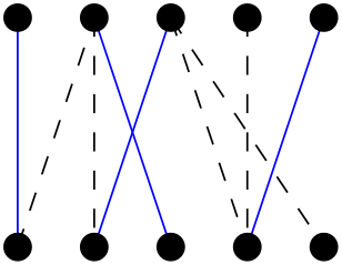
Figure17.1.3.
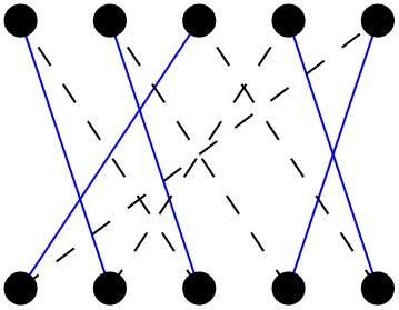
Figure17.1.4.
Solution.
There is exactly one perfect matching for this graph:
There is no perfect matching for this graph. The best we can do is to cover eight of the ten vertices. Here is one such matching:
Can you prove to yourself why there cannot be a perfect matching?
There are several perfect matchings for this graph. Here is one:
Subsection17.1.3Stable Matchings
In many cases, we want to do more than find just any matching; some matchings may be more desirable than others. This often happens when the vertices of a graph have preferences about who they will be matched with. For example, consider again the bipartite graph of people and jobs, where there is an edge connecting a person to a job when they are qualified for the job. Each person prefers some jobs over others; their preferences can be expressed as an ordered list, with their most preferred jobs at the top and their least preferred at the bottom. Each employer also has a similar list of potential employees. A bipartite graph that comes equipped with preference lists like this is called preference-labeled.
We would like to find a matching where the new hires like the job they have, and where their employers are also happy with their new hires. Obviously, we won’t always be able to give everyone their first choice of jobs or employees. However, if we are tasked with coming up with a good matching, the least we can do is try to avoid a situation where individual employees and employers are incentivized to quit or fire someone. For example, if Colby would have preferred the job opening at Google, and Google would rather have hired Colby than the person we matched them with, then Colby will quit their job and Google will replace their current employee with Colby, leaving others in the lurch. Such a matching is unstable, since individual vertices are incentivized to break their pairings; matchings that avoid this kind of instability are called stable matchings.
Stable Matchings.
A bipartite graph is preference-labeled if each vertex is given an ordering of vertices (their preferences) in the opposite part of the graph.
A stable matching in a preference-labeled bipartite graph is a matching such that there is no pair of vertices which prefer each other to their matched partners, and no vertex prefers an unmatched vertex to their matched partner.
If we want people and institutions to trust a matching we create and not go their own way, we need a way to find a stable matching. But this brings up an interesting question: does every preference-labeled bipartite graph have a stable matching?
It turns out that the answer is yes! Even better, there is an algorithm that can always find a stable matching, called the Gale-Shapley algorithm.
The Gale-Shapley Algorithm.
Choose one part of the graph to be the proposers.
Each proposer proposes to the highest vertex on their preference list which has not rejected them.
Each vertex being proposed to says "maybe" to their favorite of the vertices currently proposing to them, and rejects all other vertices currently proposing to them.
Repeat steps 2 and 3 until you reach a step where nobody is rejected. At this point, you have a stable matching.
Example17.1.5.
Let’s practice applying the Gale-Shapley algorithm to a relatively small graph, to keep things simple.
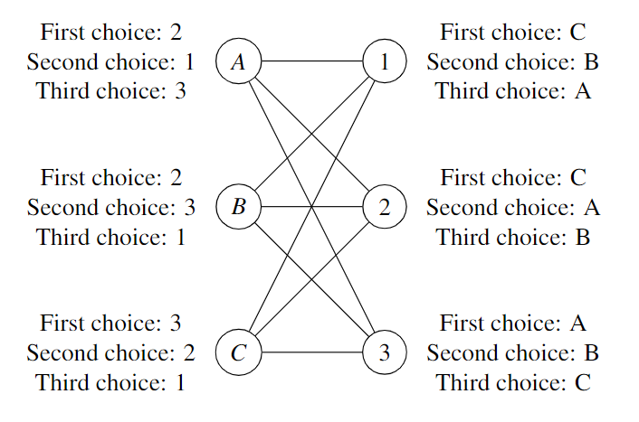
Alexis, Brandon, and Casey are graduating elementary education majors looking for teaching jobs. There are positions open at three local schools, which we’ll number 1, 2, and 3. Here is a preference-labeled graph of the prospective teachers and teaching positions:
Since all three prospective teachers are qualified for all three positions, there is an edge connecting each of them to each of the positions in the bipartite graph of people and jobs. The list next to each vertex indicates that vertex’s preferences for the vertices in the opposite part of the graph. So, for example, Alexis would prefer to work at school 2 over school 1, and school 1 over school 3. And school 1 would prefer to hire Casey over Brandon, and Brandon over Alexis.
The first step is to choose one side to be proposers. Let’s choose the teachers to propose. We’ll keep track of propositions and responses over the course of the algorithm in the tables below. For the first round of proposals, all the teachers propose to their first-choice school, since there have not yet been any rejections. So Alexis and Brandon propose to school 2 and Casey proposes to school 3. Since school 2 prefers Alexis to Brandon, it rejects Brandon and says "maybe" to Alexis. Since school 3 only received one proposal, it tells Casey "maybe". This first round can be summed up in the following table:
Propose
Reply
Alexis
2
Maybe
Brandon
2
No
Casey
3
Maybe
Next, since there was a rejection in the first round, we do another round of proposals. Since Brandon was rejected by his first choice, he will propose to his second choice, school 3. Since Alexis and Casey still have a chance with their first choices, they will propose to them again. Now school 2 only has one proposal, from Alexis, and tells her "maybe". School 3 has a proposal from Brandon and Casey, and since it prefers Brandon, it rejects Casey and says "maybe" to Brandon:
Propose
Reply
Propose
Reply
Alexis
2
Maybe
2
Maybe
Brandon
2
No
3
Maybe
Casey
3
Maybe
3
No
Since there was another rejection, we need a third round of proposals. Alexis and Brandon were not rejected, so will repeat their proposals from the last round. Casey, having been rejected by school 3, will propose to their second choice, school 2. School 2 now has a proposal from Alexis and Casey, and prefers Casey, so it will reject Alexis and tell Casey "maybe". School 3 only has a proposal from Brandon, so will tell him "maybe":
Propose
Reply
Propose
Reply
Propose
Reply
Alexis
2
Maybe
2
Maybe
2
No
Brandon
2
No
3
Maybe
3
Maybe
Casey
3
Maybe
3
No
2
Maybe
Since there was a rejection last round, we need another round of proposals. Brandon and Casey were not rejected, so they will repeat their proposals. Alexis was rejected by her first choice, so will propose to her second choice, school 1. Now each school has exactly one proposal, so they will each say "maybe":
Propose
Reply
Propose
Reply
Propose
Reply
Propose
Reply
Alexis
2
Maybe
2
Maybe
2
No
1
Maybe
Brandon
2
No
3
Maybe
3
Maybe
3
Maybe
Casey
3
Maybe
3
No
2
Maybe
2
Maybe
Since there were no rejections, we’re now done! We pair Alexis with school 1, Brandon with school 3, and Casey with school 2.
Notice that the matching reached in the example above must be stable because of the way it was chosen. If any of the prospective teachers ended up with a less-than-ideal position, they must have been rejected from all the positions that they preferred more. And the fact that they were rejected means that those schools had already been proposed to by a candidate the school preferred more, meaning that those schools ended up hiring someone they preferred over the prospective teacher in question. Therefore, there is no teacher-school pair such that the teacher prefers that school to the one they ended up with AND the school prefers that teacher to the one they ended up with. Hence, this algorithm must give a stable matching.
Example17.1.6.
Let’s try the previous example again, but this time with schools proposing, to see how that changes things. Recall the preference-labeled graph we’re using:
The table below describes the sequence of proposals and responses that should happen if we use the Gale-Shapley algorithm:
Propose
Reply
Propose
Reply
1
C
No
B
Maybe
2
C
Maybe
C
Maybe
3
A
Maybe
A
Maybe
In this case, we match school 1 with Brandon, school 2 with Casey, and school 3 with Alexis.
The matching we found this time is different. If you compared the two matchings closely, you would notice something interesting: when teachers propose, they end up in jobs they prefer more than when schools propose, and vice versa. The Gale-Shapley algorithm is biased towards the proposers. This makes sense, because the proposers get to chose what pairs are considered, and they always get to propose to the highest preference that they still have chance with. Those being proposed to, on the other hand, may never even receive a proposition from their highest preference, even if there could be a stable matching in which they are paired with their highest preference.