Subsection 11.2.1 Exponential Growth
Suppose that every year, only 10% of the fish in a lake have surviving offspring. If there were 100 fish in the lake last year, there would now be 110 fish. If there were 1000 fish in the lake last year, there would now be 1100 fish. Absent any inhibiting factors, populations of people and animals tend to grow by a percent of the existing population each year.
Let’s make a sequence listing the population of fish in a lake each year. Suppose our lake began with 1000 fish, and 10% of the fish have surviving offspring each year. Since we start with 1000 fish, \(P_0 = 1000.\) How do we calculate the population for the next year? The new population will be the old population, plus an additional 10%. Symbolically, the next term is:
\begin{equation*}
P_0 + 0.10P_0
\end{equation*}
Notice this could be condensed to a shorter form by factoring:
\begin{equation*}
P_0 + 0.10P_0 = 1P_0 + 0.10P_0 = (1+0.10)P_0 = 1.10P_0
\end{equation*}
While 10% is the growth rate, 1.10 is the growth multiplier. Notice that 1.10 can be thought of as “the original 100% plus an additional 10%”.
So we could calculate the fish population after one year in the following way:
\begin{equation*}
1.10(1000) = 1100
\end{equation*}
We can also calculate the population in later years like this:
\begin{equation*}
\text{After 2 years: } 1.10P_1 = 1.10(1100) = 1210
\end{equation*}
\begin{equation*}
\text{After 3 years: } 1.10P_2 = 1.10(1210) = 1331
\end{equation*}
Notice that in the first year, the population grew by 100 fish, in the second year, the population grew by 110 fish, and in the third year the population grew by 121 fish. While there is a constant percentage growth, the actual number of fish added is increasing each year.
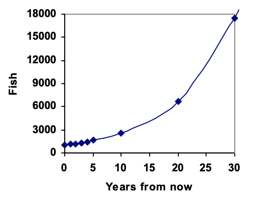
Graphing these values we see that this growth doesn’t quite appear linear.
To get a better picture of how this percentage-based growth affects things, we need a faster way to calculate values further out in the future. Just as we found a faster way to do repeated addition with linear models, here we need a quick way to do repeated multiplication.
Like we did for the linear model, let’s start building each term of the sequence from the initial term, and see if we can find a pattern:
After 1 year: \(1.10P_0 = 1.10(1000)\)
After 2 years: \(1.10(1100) = 1.10(1.10(1000)) = 1.10^2(1000)\)
After 3 years: \(1.10(1210) = 1.10(1.10(1.10(1000))) = 1.10^3(1000)\)
After 4 years: \(1.10(1331) = 1.10(1.10(1.10(1.10(1000)))) = 1.10^4(1000)\)
It makes sense that we end up using exponents here. Just as multiplication is repeated addition, exponentiation is repeated multiplication.
Observing a pattern, we can generalize to a formula for the population (\(P\)) of fish after any number (\(n\)) of years: \(P = 1.10^n(1000)\) or equivalently \(P = (1000)1.10^n\text{.}\)
From this, we can quickly calculate the number of fish in 10, 20, or 30 years:
After 10 years: \((1000)1.10^{10} = 2594\)
After 20 years: \((1000)1.10^{20} = 6727\)
After 30 years: \((1000)1.10^{30} = 17449\)
Adding these values to our graph reveals a shape that is definitely not linear. If our fish population had been growing linearly, by 100 fish each year, the population would have only reached 4000 in 30 years compared to almost 18000 with this percent-based growth, called exponential growth.
In exponential growth, the population grows proportional to the size of the population, so as the population gets larger, the same percent growth will yield a larger numeric growth.
Exponential Sequences.
A sequence is exponential if it changes by a common percentage.
We call the common percentage the percent growth rate, which in decimal form is designated as \(r\text{.}\) In the case of our fish population, \(r = 0.10\text{.}\)
The common ratio or growth multiplier for an exponential sequence is the number you multiply each term by to get the next term. The growth multiplier is always equal to \(1+r\text{.}\) In the case of our fish population, the growth multiplier is \(1.10\text{.}\)
If \(r\) is positive (equivalently, if the growth multiplier is greater than 1), the sequence is increasing and we say that it exhibits exponential growth. If \(r\) is negative (equivalently, if the growth multiplier is less than 1), the sequence is decreasing and we say that it exhibits exponential decay.
If a quantity starts at size \(P_0\) and grows by \(R\)% (written as a decimal, \(r\)) every time period, then the quantity \(P\) after \(n\) time periods can be determined using this formula:
\(\hspace{2.5in} P = P_0(1+r)^n\)
Example 11.2.1.
Between 2007 and 2008, Olympia, WA grew almost 3% to a population of 245 thousand people. If this growth rate was to continue, what would the population of Olympia be in 2014?
As we did before, we first need to define what year will correspond to \(n=0\text{.}\) Since we know the population in 2008, it would make sense to have 2008 correspond to \(n=0\text{,}\) so \(P_0 = 245,000\text{.}\) The year 2014 would then be \(n=6\text{.}\)
We know the growth rate is 3%, giving \(r\)=0.03. So the growth multiplier is 1.03.
Then we can calculate the population when \(n=6\) like this:
\begin{equation*}
345,000(1.03)^6 = 1.19405(245,000) = 292,542.25
\end{equation*}
The model predicts that in 2014, Olympia would have a population of about 293 thousand people.
Evaluating exponents on the calculator.
To evaluate expressions like \((1.03)^6\) it will be easier to use a calculator than multiply 1.06 by itself six times. Most scientific calculators have a button for exponents. It is typically either labeled like:
^, \(y^x\text{,}\) or \(x^y\)
To evaluate \(1.03^6\text{,}\) we’d type 1.03 ^ 6 or 1.03 \(y^x\) 6. Try it out - you should get an answer around 1.1940523.
Exploration 11.2.1.
India is the second most populous country in the world, with a population in 2008 of about 1.14 billion people. The population is growing by about 1.34% each year. If this trend continues, what will India’s population grow to by 2020?
Solution.
Using \(n=0\) corresponding with 2008, in 2020 \(n\) will be \(12\text{.}\) Then
\begin{equation*}
1.14(1+0.0314)^{12} = \text{about } 1.137 \text{ billion people in 2020}
\end{equation*}
Example 11.2.2.
A friend is using the equation \(P = 4600(1.072)^n\) to predict the annual tuition at a local college. She says the formula is based on years after 2010. What does this equation tell us?
In the equation, \(P_0\) = 4600, which is the starting value of the tuition when \(n = 0\text{.}\) This tells us that the tuition in 2010 was $4,600.
The growth multiplier is 1.072, so the growth rate is 0.072, or 7.2%. This tells us that the tuition is expected to grow by 7.2% each year.
Putting this together, we could say that the tuition in 2010 was $4,600, and is expected to grow by 7.2% each year.
Example 11.2.3.
In 1990, the residential energy use in the US was responsible for 962 million metric tons of carbon dioxide emissions. By the year 2000, that number had risen to 1182 million metric tons. If the emissions grow exponentially and continue at the same rate, what will the emissions grow to by 2050?
Similar to before, we will correspond \(n = 0\) with 1990, as that is the year for the first piece of data we have. That will make \(P_0 = 962\) (million metric tons of CO2). In this problem, we are not given the growth rate, but instead are given that the tenth term of the sequence is 1182.
When \(n=10\text{,}\) plugging what we know into our formula gives us
\begin{equation*}
1182 = 962(1+r)^{10}
\end{equation*}
We can now solve this equation for the growth rate \(r\text{.}\) Start by dividing by 962.
\begin{align*}
\frac{1182}{962} \amp = (1+r)^{10} \amp \amp \text{Take the 10th root of both sides} \\
\sqrt[10]{\frac{1182}{962}} \amp = 1+r \amp\amp \text{Subtract 1 from both sides} \\
r \amp = \sqrt[10]{\frac{1182}{962}}-1 = 0.0208 = 2.08\%
\end{align*}
So if the emissions are growing exponentially, they are growing by about 2.08% per year. We can now predict the emissions in 2050 by plugging \(r = 0.0208\) and \(n = 60\) into our formula:
\(962(1+0.0208)^{60} = 3308.4\) million metric tons of CO\(_2\) in 2050.
Rounding.
As a note on rounding, notice that if we had rounded the growth rate to 2.1%, our calculation for the emissions in 2050 would have been 3347. Rounding to 2% would have changed our result to 3156. A very small difference in the growth rates gets magnified greatly in exponential growth. For this reason, it is recommended to round the growth rate as little as possible.
If you need to round, keep at least three significant - numbers after any leading zeros. So 0.4162 could be reasonably rounded to 0.416. A growth rate of 0.001027 could be reasonably rounded to 0.00103.
Evaluating roots on the calculator.
In the previous example, we had to calculate the 10th root of a number. This is different than taking the basic square root, \(\sqrt{}\text{.}\) Many scientific calculators have a button for general roots. It is typically labeled like: \(\sqrt[n]{} \text{, } \sqrt[x]{} \text{, or } \sqrt[y]{x} \)
To evaluate the 3rd root of 8, for example, we’d either type \(3 \sqrt[x]{} 8 \) or \(8 \sqrt[y]{x} 3\text{,}\) depending on the calculator. Try it on yours to see which to use - you should get an answer of 2.
If your calculator does not have a general root button, all is not lost. You can instead use the property of exponents which states that \(\sqrt[n]{a} = a^{\frac{1}{n}}\text{.}\) So to compute the 3rd root of 8, you could use your calculator’s exponent key to calculate \(8^{\frac{1}{3}}\text{.}\) To do this, type: \(8 y^x (1 \div 3)\text{.}\)
The parentheses tell the calculator to divide 1/3 before doing the exponent.
Exploration 11.2.2.
The number of users on a social networking site was 45 thousand in February when they officially went public, and grew to 60 thousand by October. If the site is growing exponentially, and growth continues at the same rate, how many users should they expect two years after they went public?
Solution.
Here we will measure \(n\) in months rather than years, with \(n = 0\) corresponding to the February when they went public. This gives \(P_0 = 45\) thousand. October is 8 months later, so the eighth term is \(60\)
\begin{equation*}
60 = 45(1+r)^8
\end{equation*}
\begin{equation*}
\frac{60}{45} = (1+r)^8
\end{equation*}
\begin{equation*}
\sqrt[8]{\frac{60}{45}} = 1 + r
\end{equation*}
\begin{equation*}
r = \sqrt[8]{\frac{60}{45}} -1 = 0.0366 \text{ or } 3.66\%
\end{equation*}
So our general equation is \(P = 45(1.0366)^n\text{.}\) Predicting 24 months (2 years) after they went public:
\begin{equation*}
45(1.0366)^{24} = 106.63 \text{ thousand users}
\end{equation*}
Example 11.2.4.
Looking back at the last example, for the sake of comparison, what would the carbon emissions be in 2050 if emissions grow linearly at the same rate?
Again we will get \(n = 0\) corresponds with 1990, giving \(P_0 = 962\text{.}\) To find the common difference \(d\text{,}\) we could take the same approach as earlier, noting that the emissions increased by 220 million metric tons in 10 years, giving a common difference of 22 million metric tons each year.
Alternatively, we could use an approach similar to that which we used to find the exponential equation. When \(n = 10\text{,}\) we know that emissions were at 1182 million metric tons, so the linear equation looks like:
\begin{equation*}
1182 = 962 + 10d
\end{equation*}
We can now solve this equation for the common difference, d
\begin{equation*}
1182-962 = 10d
\end{equation*}
\begin{equation*}
220 = 10d
\end{equation*}
\begin{equation*}
d = 22
\end{equation*}
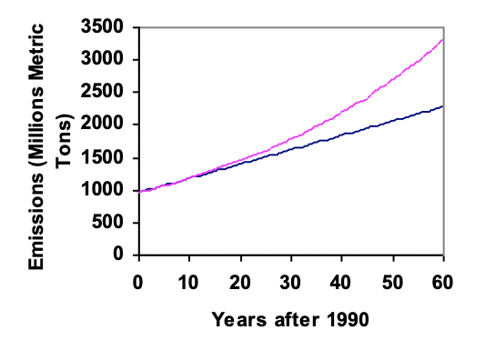
This tells us that if the emissions are changing linearly, they are growing by 22 million metric tons each year. Predicting the emissions in 2050, we get
\begin{equation*}
962 + 22(60) = 2282 \text{ million metric tons}
\end{equation*}
You will notice that this number is substantially smaller than the prediction from the exponential growth model. Calculating and plotting more values helps illustrate the differences.