Subsection3.3.1Continuous probability distributions
At the beginning of this chapter we discussed discrete probability distributions which summarized the probabilities of experiments with a finite number of possible outcomes. However, in some situations, it makes sense to consider the outcomes of an experiment to fall within a continuous range of outcomes, in which case there are infinitely many possible outcomes.
Consider again the probability distribution from Exploration 3.1.3, regarding commute time. In that Exploration, we considered the outcomes to be integer numbers of minutes for simplicity’s sake, but we could add more detail. A given commute might take closer to 23.25 minutes than 23 minutes, a level of precision that we ignored. In theory, your commute could take any number of minutes, including decimal numbers of minutes like 21.326 or even 26.202002000200002.... Although we would never be able to measure your travel time with an infinite amount of precision, it makes sense to say that your actual travel time could be any of the infinitely-many real numbers within a reasonable range; all of these numbers are possible outcomes.
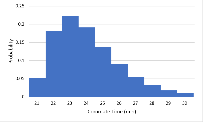
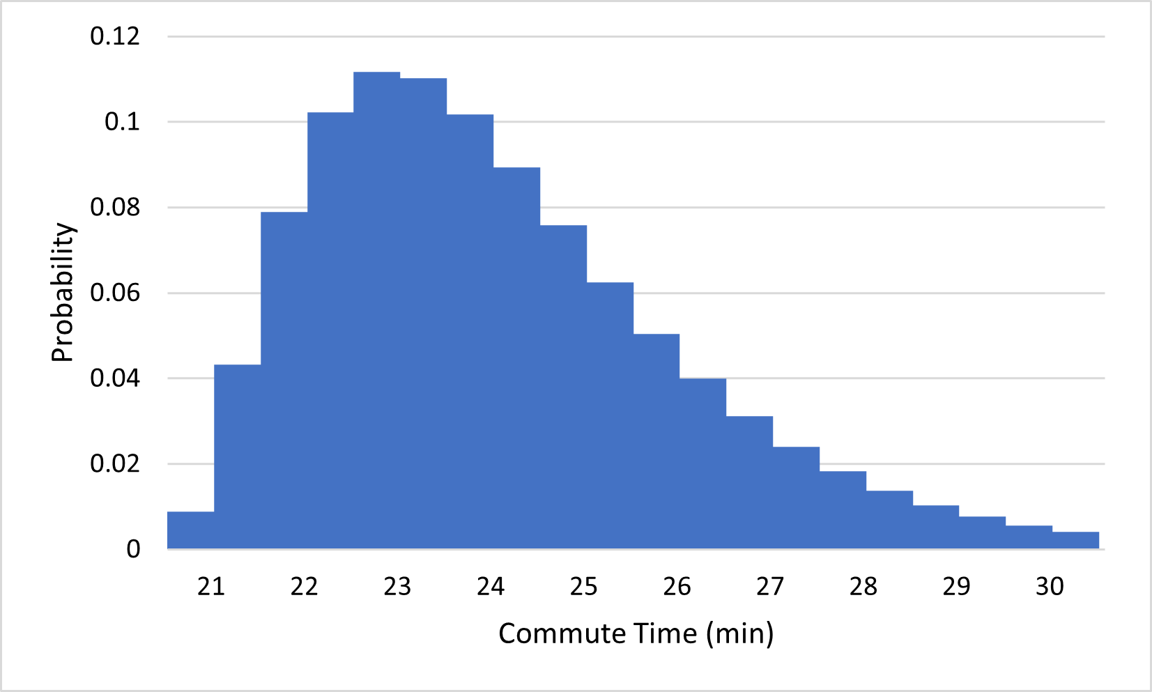
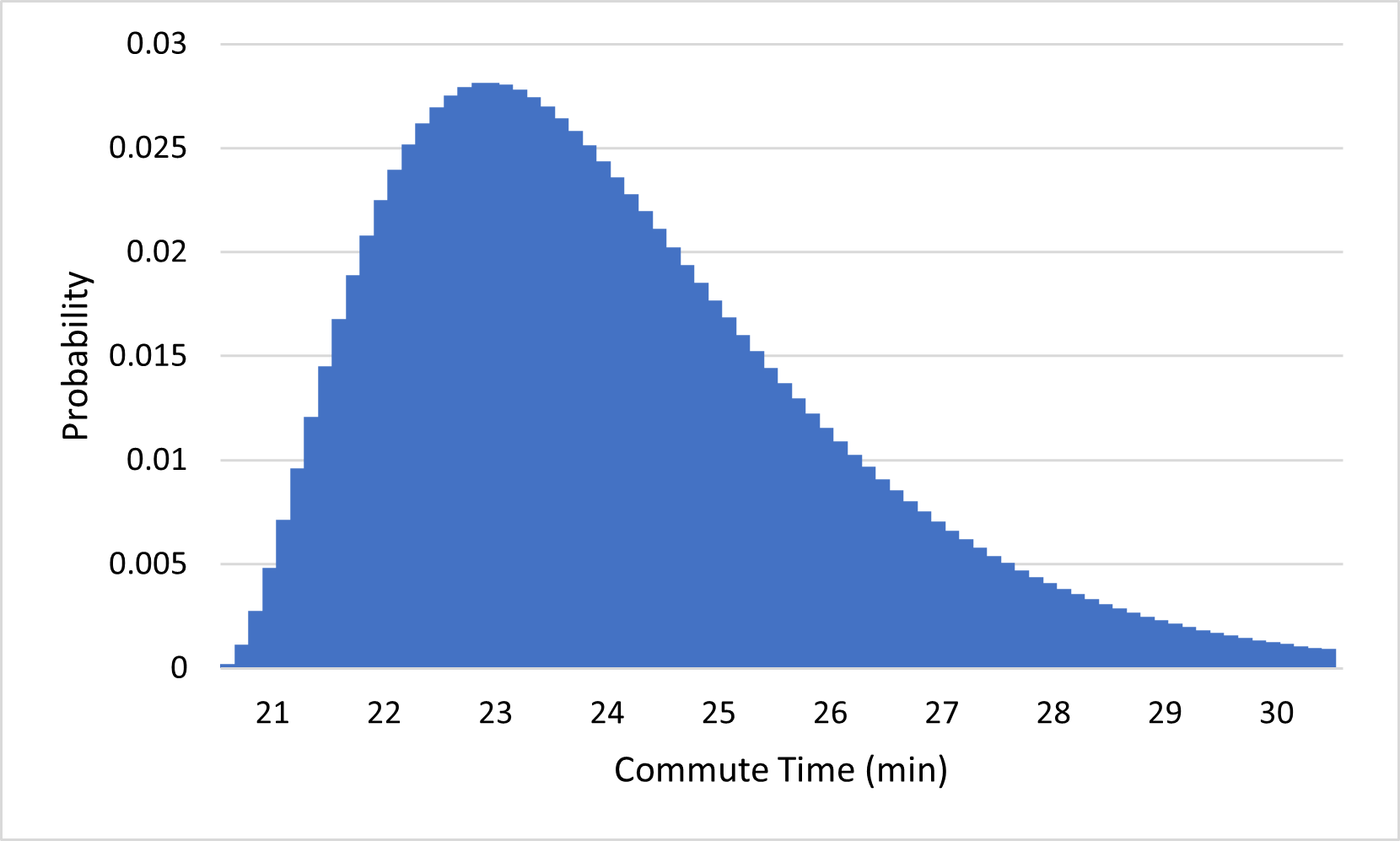
There is an interesting consequence for probability when the outcomes of an experiment span a continuous interval of numbers: the probability of any given outcome is typically 0. To get some intuition for why this should be true, consider what happens to the commute time probability distribution if we start splitting outcomes into more precise categories, from the nearest minute, to the nearest half-minute, to the nearest quarter-minute, and so on:
(a)Measuring commute time to the nearest minute
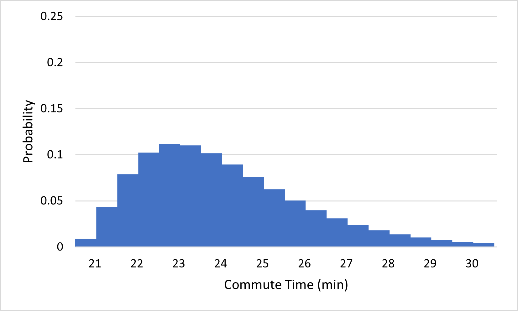
(b)...to the nearest half-minute
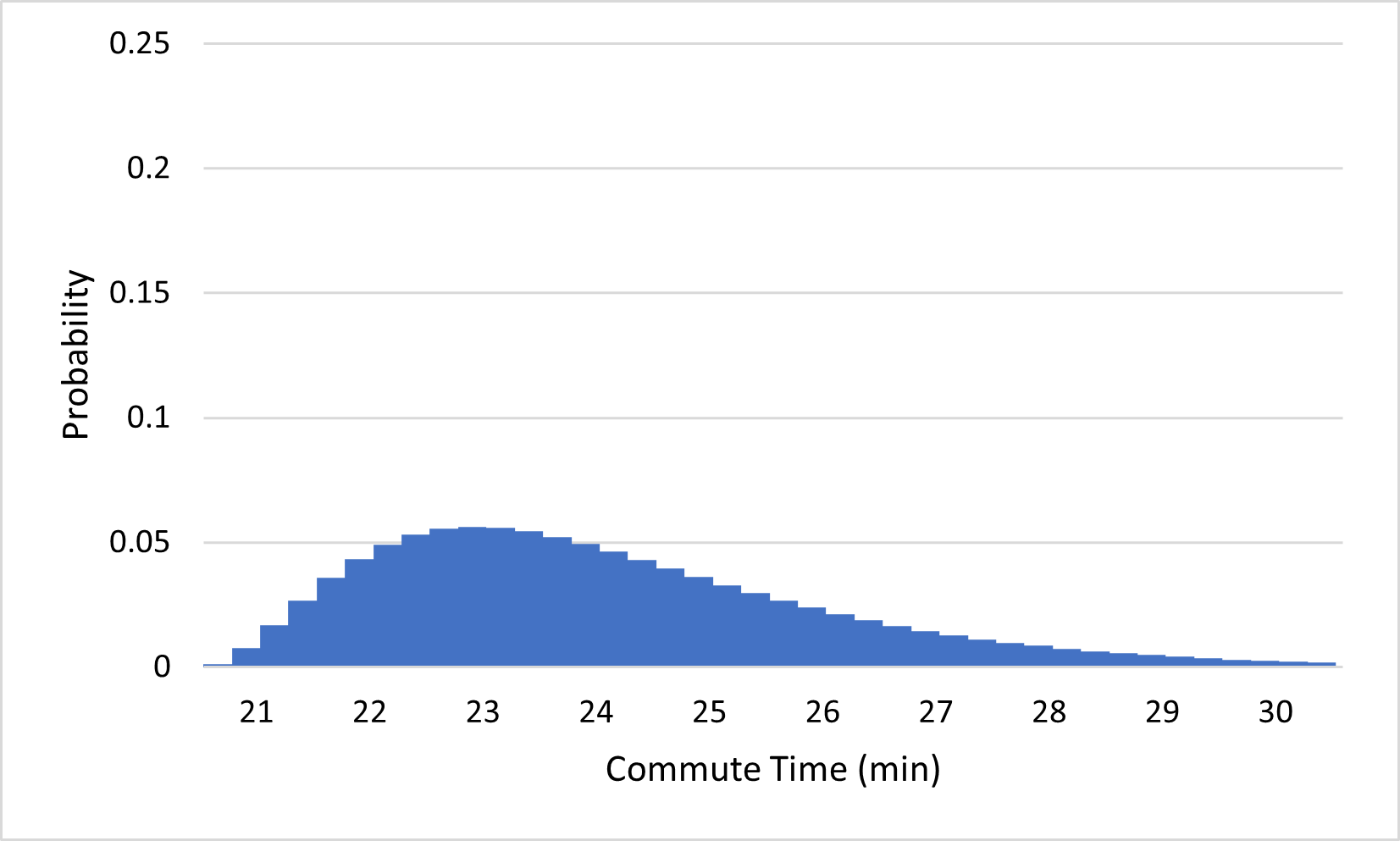
(c)...to the nearest quarter-minute
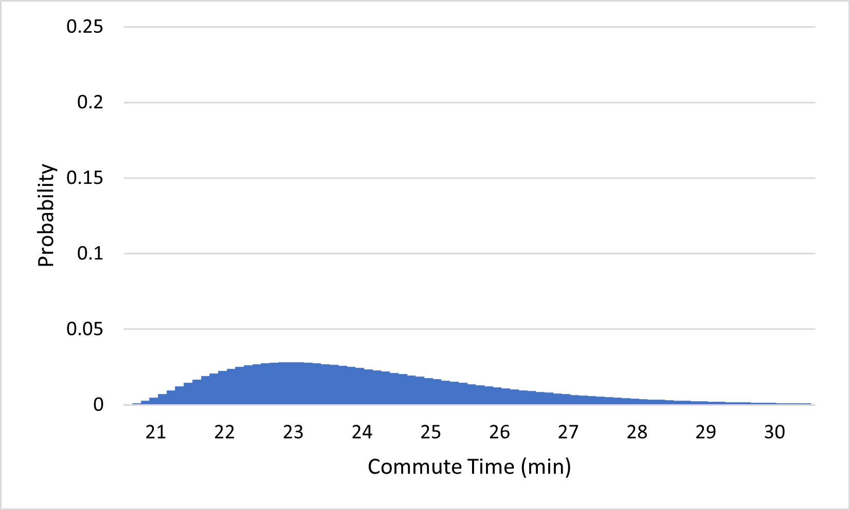
(d)...to the nearest eighth-minute
Figure3.3.1.Splitting the commute time distribution into more and more precise outcomes.
Notice that the probabilities of the outcomes keep getting closer and closer to 0 as we add more precision to our outcomes. This makes sense; it is much less likely that you will arrive within one second of your expected arrival time than that you will arrive within one minute of it. If we continue this process indefinitely, the probabilities approach 0. Since the probability of arriving exactly 23 minutes after you left, for example, must be even less than that of arriving within one millisecond of 23 minutes, or within any tiny amount of error, the probability of your commute taking exactly 23 minutes must be 0. Similarly, the probability of any number being the exact amount of time your commute takes is 0.
Because each outcome of this experiment has a probability of 0, listing the probability of each outcome or drawing a graph of the probability of each outcome isn’t going to be useful to us like it was with discrete probability distributions. However, given any interval of possible outcomes, there may be some non-zero probability that the outcome of the experiment falls within that interval; for example, there is some non-zero probability that your commute takes between 24 and 27 minutes, and a smaller probability that it takes between 24.5 and 26.15 minutes. Our goal will be to convey the probability corresponding to any interval of minutes, rather than a particular number of minutes.
You may have noticed in Figure 3.3.1 that, although the individual probabilities are all getting smaller, the general shapes of the distributions all look similar. To see this more clearly, here’s what each of the distributions in Figure 3.3.1 looks like if we scale their vertical axes so that they all appear to have the same height:
(a)Measuring commute time to the nearest minute
(b)...to the nearest half-minute
(c)...to the nearest quarter-minute
(d)...to the nearest eighth-minute
Figure3.3.2.Scaling each vertical axis so that each distribution appears to have the same height.
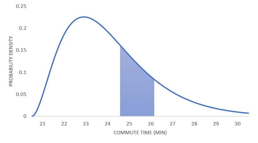
If we continue this process of splitting the distribution into more and more precise outcomes, and keep scaling the vertical axis to keep the height of the distributions constant, these graphs will approach a smooth curve, as in Figure 3.3.3. This curve is called the probability density function, or the continuous probability distribution for the experiment. The probability density function will tell us the probability corresponding to any interval.
Figure3.3.3.The probability density function for your commute time. The area of the shaded region is the probability that your commute takes between 24.5 and 26.15 minutes.
Notice that, in each of the bar graphs representing a finite probability distribution, the proportion of area in the graph over a given interval roughly represents the probability that the outcome of the experiment will fall within that interval. For example, the proportion of area in the bars past the 27 minute mark represents the probability that your commute takes at least 27 minutes. In the same way, given any interval of minutes, the probability that your commute time falls within that interval is the proportion of area under the probability density function over that interval. To make things simpler, we scale the density function so that the total area under the curve is 1, making area equal to probability.
Probability Density Functions.
A probability density function (also known as a continuous probability distribution) is a curve that fully describes the probabilities involved in an experiment where the collection of outcomes is a continuous interval.
The probability of any given outcome of such an experiment is typically 0, so we only measure the probability that the result of the experiment falls within an interval of outcomes.
Given an interval of outcomes, the probability associated to the interval is the area under the probability density function over that interval.
The total area under a probability density function is 1, since this is the probability that any outcome in the interval of all possible outcomes occurs.
Exploration3.3.1.
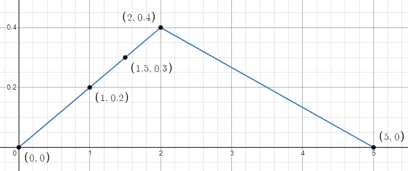
Suppose a computer program outputs a random number between 0 and 5 with the following probability density function:
What is the probability that the output is greater than 2?
What is the probability that the output is between 1 and 2?
What is the probability that the output is at least 1.5?
Solution.
This probability is represented by the area under the curve from 2 to 5 on the horizontal axis, which is the area of the triangle with vertices \((2,0)\text{,}\)\((2,0.4)\text{,}\) and \((5,0)\text{.}\) It has a base of 3 and a height of 0.4, so its area is \(\frac{1}{2} \cdot 3 \cdot 0.4 = 0.6\text{.}\) Therefore, the probability that the output is greater than 2 is 0.6, or 60%.
This probability is represented by the area of the trapezoid with vertices at \((1,0)\text{,}\)\((1,0.2)\text{,}\)\((2,0.4)\text{,}\) and \((2,0)\text{.}\) One way to find its area is to split it into a triangle with base 1 and height 0.2, and a rectangle with base 1 and height 0.2, making the total area \(\frac{1}{2} \cdot 1 \cdot 0.2 + 1 \cdot 0.2 = 0.3\text{.}\) Therefore, the probability that the output is between 1 and 2 is 0.3 or 30%.
This probability is represented by the area of the quadrilateral with vertices \((1.5,0)\text{,}\)\((1.5,0.3)\text{,}\)\((2,0.4)\text{,}\) and \((5,0)\text{.}\) However, it is probably easiest to find this area by subtracting the area under the curve between 0 and 1.5 from the total area under the curve, which we know to be 1. The area under the curve between 0 and 1.5 is the area of a triangle with vertices \((0,0)\text{,}\)\((1.5,0.3)\text{,}\) and \((1.5,0)\text{,}\) which has a base of 1.5 and height of 0.3, making its area \(\frac{1}{2} \cdot 1.5 \cdot 0.3 = 0.225\text{.}\) So the area under the curve from 1.5 to 5, and therefore the probability that the output is at least 1.5, is \(1 - 0.225 = 0.775\text{,}\) or 77.5%.
Exploration3.3.2.
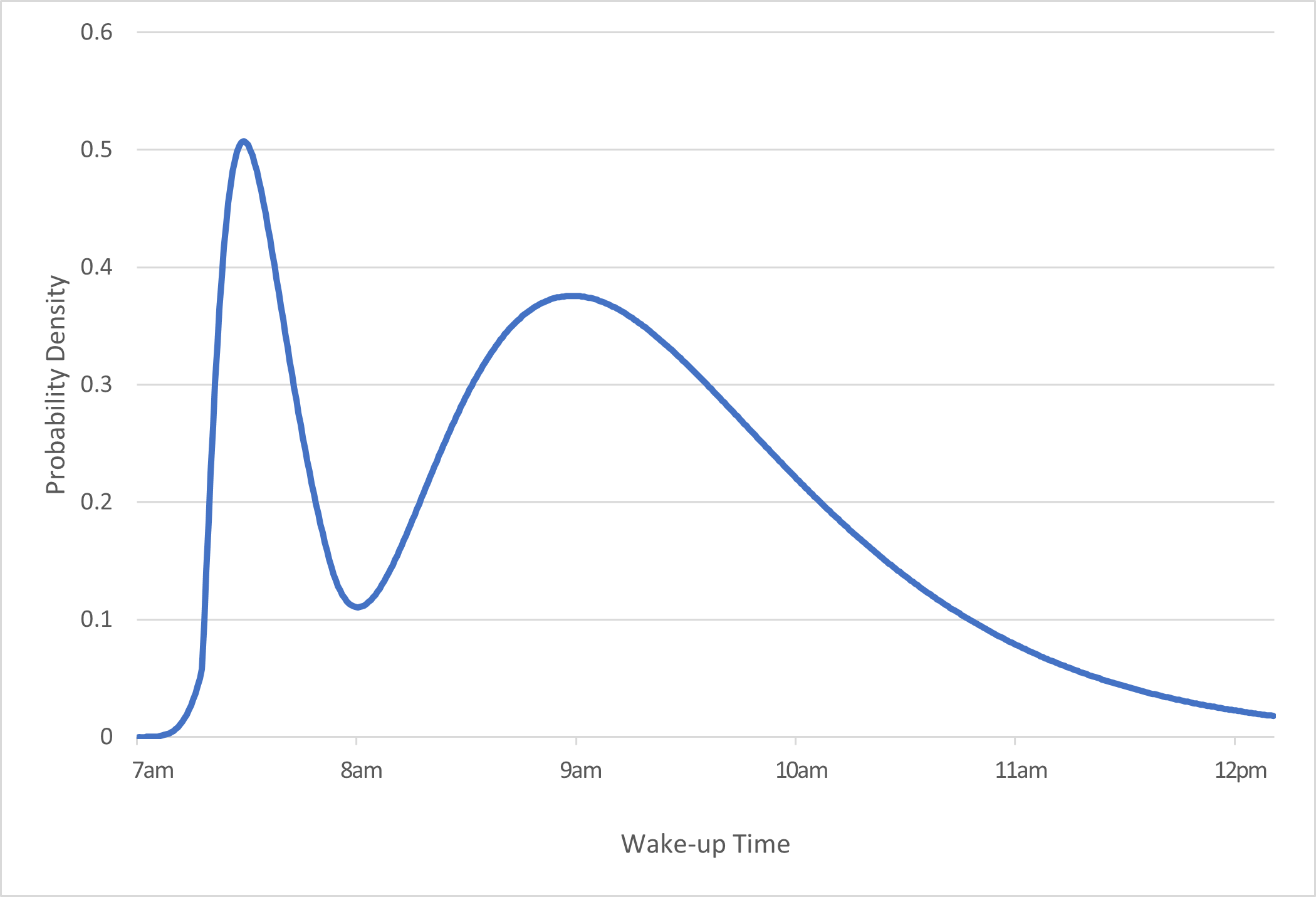
Riley sometimes works a morning shift and sometimes works an afternoon shift. Below is a probability density function for the time they wake up in the morning.
Is Riley more likely to wake up before or after 8am?
Distributions that have multiple peaks like this one are called bimodal. Based on the context of the problem, why do you think this distribution is bimodal?
The first peak is taller and thinner, and the second peak is shorter and wider. What do you think accounts for these differences in the width and height of the two peaks?
Solution.
Although the peak in the graph before 8am is higher than the peak after, the area under the curve after 8am is larger, since the second peak is much wider. Since area represents probability, this means that Riley is more likely to wake up after 8am.
It is probably bimodal because Riley sometimes needs to get up for work early in the morning (accounting for the first peak) and sometimes doesn’t, and sleeps in more (accounting for the second peak). Based on the answer to the previous question, Riley likely works afternoon shifts more often than morning shifts.
The fact that the first peak is tall and skinny means that a relatively large amount of probability is distributed over a short time period. In other words, on days that Riley gets up early for their morning shift, they probably set an alarm around 7:15am and wake up to it fairly quickly and consistently in order to avoid being late for work. The fact that the second peak is shorter and wider means that on days that Riley doesn’t work a morning shift, their wake-up time is not quite as consistent; although they most often wake up around 9am, they also often sleep in.
Exploration3.3.3.
Can the height of a probability density function go above 1? Explain why or why not.
Solution.
The height can go above 1. Since the height of the function does not represent probability, there is no limit on the height of a probability density function. It is true that the area under a probability density function must equal 1, and therefore if there is a very high peak, it must be very thin in order to avoid accumulating more than 1 unit of area under the curve.