Subsection4.2.1Sample means and standard deviation
If bags of chips are produced with an average weight of 15 oz and a standard deviation of 0.1 oz, what is the probability that the average weight of 30 bags will be within 0.1 oz of the mean? The answer is not 68%! To answer this question we must visualize and understand what is called the sampling distribution of a sample mean.
It is not always reasonable to look at the entire population of data. Sometimes we need to take a sample. How do we know that a sample can tell us reliable information about a larger population?
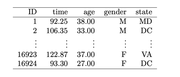
In this section we consider a data set which represents all 19,961 runners who finished the 2017 Cherry Blossom 10 mile run in Washington, DC. 1
www.cherryblossom.org
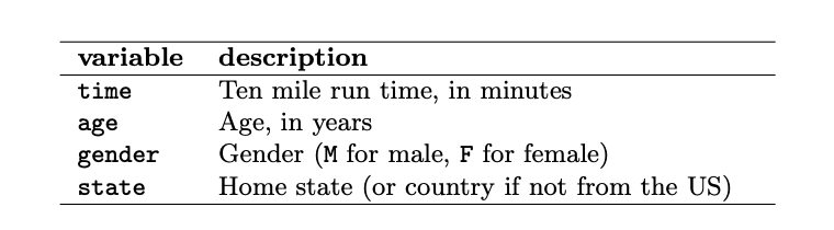
. Part of this data is shown in figure 4.7 and the variables are described in figure 4.8.
Figure4.2.1.Four observations from the 2017 Cherry Blossom 10 mile run
Figure4.2.2.Variables and their descriptions from the 2017 Cherry Blossom 10 mile run
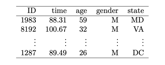
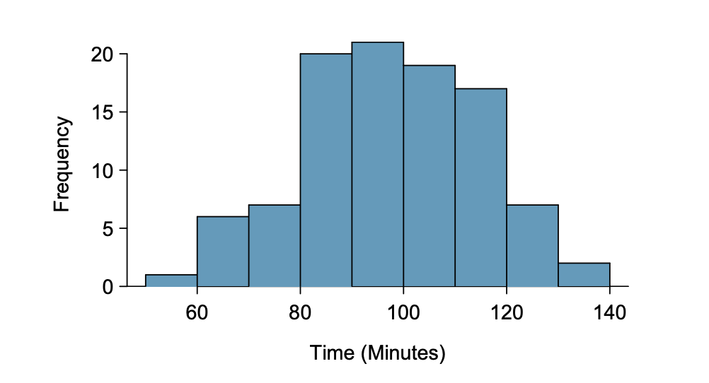
These data are special because they include the results for the entire population of runners who finished the 2017 Cherry Blossom Run. We took a simple random sample of 100 runners from this population, which is represented in Figure 4.9. A histogram summarizing the time variable in the sample data set is shown in Figure 4.10.
Figure4.2.3.Three observations for the sample data set, which represents a simple random sample of 100 runners from the 2017 Cherry Blossom Run
Figure4.2.4.Histogram of time for a single sample of size 100. The average of the sample is in the mid-90s (95.61 minutes) and the standard deviation of the sample s \(\approx\) 17 minutes.
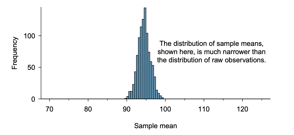
From the random sample represented in figure 4.9, we found the average time it takes to run 10 miles is 95.61 minutes. Suppose we take another random sample of 100 individuals and take its mean: 95.30 minutes. Suppose we took another (93.43 minutes) and another (94.16 minutes), and so on. If we do this many many times – which we can do only because we have the entire population data set – we can build up a sampling distribution for the sample mean when the sample size is 100, shown in Figure 4.11
Sampling Distribution.
The sampling distribution represents the distribution of the point estimates based on samples of a fixed size from a certain population. It is useful to think of a point estimate as being drawn from such a distribution. Understanding the concept of a sampling distribution is central to understanding statistical inference.
The sampling distribution shown in Figure 4.11 is unimodal and approximately symmetric. It is also centered exactly at the true population mean: \(\mu\) = 94.52. Intuitively, this makes sense. The sample mean should be an unbiased estimator of the population mean. Because we are considering the distribution of the sample mean, we will use \(X\) = 94.52 to describe the true mean of this distribution.
Figure4.2.5.A histogram of 1000 sample means for run time, where the samples are of size n = 100. This histogram approximates the true sampling distribution of the sample mean, with mean \(X\) and standard deviation \(s\text{.}\)
We can see that the sample mean has some variability around the population mean, which can be quantified using the standard deviation of this distribution of sample means. The standard deviation of the sample mean tells us how far the typical estimate is away from the actual population mean, 94.52 minutes. It also describes the typical error of a single estimate, and is denoted by the symbol \(s\text{.}\)
Standard deviation of an estimate.
The standard deviation associated with an estimate describes the typical error or uncertainty associated with the estimate.
Example4.2.6.
Looking at figures 4.10 and 4.11, we see that the standard deviation of the sample mean with n = 100 is much smaller than the standard deviation of a single sample. Interpret this statement and explain why it is true.
The variation from one sample mean to another sample mean is much smaller than the variation from one individual to another individual. This makes sense because when we average over 100 values, the large and small values tend to cancel each other out. While many individuals have a time under 90 minutes, it would be unlikely for the average of 100 runners to be less than 90 minutes.
Example4.2.7.
Would you rather use a small sample or a large sample when estimating a parameter? Why?
Consider two random samples: one of size 10 and one of size 1000. Individual observations in the small sample are highly influential on the estimate while in larger samples these individual observations would more often average each other out. The larger sample would tend to provide a more accurate estimate.
Using your reasoning from part 1, would you expect a point estimate based on a small sample to have smaller or larger standard deviation than a point estimate based on a larger sample?
If we think an estimate is better, we probably mean it typically has less error. Based on part 1, our intuition suggests that a larger sample size corresponds to a smaller standard deviation.
We can calculate the standard deviation of the sample means using the following formula:
\begin{equation*}
s = \frac{\sigma}{\sqrt{n}}
\end{equation*}
where \(\sigma\) is the standard deviation of the parent population and \(n\) is the number of observations in the sample.
Example4.2.8.
The average of the runners’ ages is 35.05 years with a standard deviation of \(\sigma\) = 8.97. A simple random sample of 100 runners is taken.
What is the standard deviation of the sample mean?
Using the equation above, we find that \(s = \frac{8.97}{\sqrt{100}} = \frac{8.97}{10} = 0.897.\)
Would you be surprised to get a sample of size 100 with an average of 36 years?
It would not be surprising. 36 years is about 1 standard deviation from the true mean of 35.05. Based on the 68-95-99.7 rule, we would get a sample mean at least this far away from the true mean approximately 100% − 68% = 32% of the time.
Subsection4.2.2Normal Distributions and Confidence Intervals
The site fivethirtyeight.com regularly forecasts support for each candidate in Congressional races, i.e. races in the US House of Representatives and the US Senate. In addition to point estimates, they report confidence intervals. What are confidence intervals, and how do we interpret them?
A point estimate provides a single plausible value for a parameter. However, a point estimate isn’t perfect and will have some standard error associated with it. When estimating a parameter, it is better practice to provide a plausible range of values instead of supplying just the point estimate.
Point estimates only approximate the population parameter. How can we quantify the expected variability in a point estimate? The variability in the distribution of the point estimate is given by its standard deviation. If we know the population proportion, we can calculate the standard deviation of the point estimate.
The standard deviation for the question "What proportion or fraction of people favor alternative A" is given by the formula \(\sigma = \sqrt{p(1-p)}\) where \(p\) is the population proportion, or the fraction of the population, that favors alternative A. Then the standard deviation for the point estimate or sample of size \(N\) is
\begin{equation*}
s = \frac{\sigma}{\sqrt{N}} = \sqrt{\frac{p(1-p)}{N}}
\end{equation*}
A plausible range of values for the population parameter is called a confidence interval. Using only a point estimate is like fishing in a murky lake with a spear, and using a confidence interval is like fishing with a net. We can throw a spear where we saw a fish, but we will probably miss. On the other hand, if we toss a net in that area, we have a good chance of catching the fish.
If we report a point estimate, we probably will not hit the exact population parameter. On the other hand, if we report a range of plausible values – a confidence interval – we have a good shot at capturing the parameter.
A point estimate is our best guess for the value of the parameter, so it makes sense to build the confidence interval around that value. The standard error is a measure of the uncertainty associated with the point estimate.
Example4.2.9.
How many standard errors should we extend above and below the point estimate if we want to be 95% confident of capturing the true value?
First, we observe that the area under the standard normal curve that is within two standard deviations of the mean is 95%. When conditions for a normal model are met, the point estimate we observe will be within 2 standard deviations of the true value about 95% of the time. Thus, if we want to be 95% confident of capturing the true value, we should go 2 standard errors on either side of the point estimate.
Note that this 2 standard deviations is approximate - statisticians use 1.96 exactly!
Constructing a 95% confidence interval using a normal mdoel.
When the sampling distribution of a point estimate can reasonably be modeled as normal, a 95% confidence interval for the unknown parameter can be constructed as:
point estimate +/- 2 x \(s\)
Example4.2.10.
Suppose that in a sample, we find that 15% of people in a community support a new ballot measure. The standard deviation \(s\) for this point estimate was calculated to be \(s\) = 0.04. Assuming that conditions for a normal model are met, construct and interpret a 95% confidence interval.
point estimate +/- 2 x \(s\)
0.15 +/- 2 x 0.04
(0.0716,0.2284)
We are 95% confident that the true percent of people who favor the ballot measure is between 7.16% and 22.84%.