Subsection 3.1.1 Introduction
The probability of a specified event is the chance or likelihood that it will occur. There are several ways of viewing probability. One would be experimental in nature, where we repeatedly conduct an experiment. Suppose we flipped a coin over and over and over again and it came up heads about half of the time; we would expect that in the future whenever we flipped the coin it would turn up heads about half of the time. When a weather reporter says “there is a 10% chance of rain tomorrow,” she is basing that on prior evidence; that out of all days with similar weather patterns, it has rained on 10 out of 100 (or 1 out of 10) of those days.
Another view would be subjective in nature, in other words an educated guess. If someone asked you the probability that the Seattle Mariners would win their next baseball game, it would be impossible to conduct an experiment where the same two teams played each other repeatedly, each time with the same starting lineup and starting pitchers, each starting at the same time of day on the same field under precisely the same conditions. Since there are so many variables to take into account, someone familiar with baseball and with the two teams involved might make an educated guess that there is a 75% chance they will win the game; that is, if the same two teams were to play each other repeatedly under identical conditions, the Mariners would win about three out of every four games. But this is just a guess, with no way to verify its accuracy, and depending upon how educated the educated guesser is, a subjective probability may not be worth very much.
We will return to the experimental and subjective probabilities from time to time, but in this course we will mostly be concerned with theoretical probability, which is defined as follows: Suppose there is a situation with \(n \) equally likely possible outcomes and that \(m \) of those \(n \) outcomes correspond to a particular event; then the probability of that event is defined as \(\frac{m}{n} \text{.}\)
If you have learned about probability in previous classes, it was probably theoretical probability. For example, if we think about the probability of tossing a head on a fair coin from a theoretical perspective, then tossing a fair coin has 2 equally likely outcomes (\(n=2\)) and heads is one of those outcomes (\(m=1\)), so the probability of tossing a head is \(\frac{1}{2}\text{.}\) More examples are below.
Subsection 3.1.2 Basic Concepts
If you roll a die, pick a card from deck of playing cards, or randomly select a person and observe their hair color, we are executing an experiment or procedure. In probability, we look at the likelihood of different outcomes. We begin with some terminology.
Events and Outcomes.
The result of an experiment is called an outcome. Outcomes must be disjoint, meaning that two different outcomes cannot happen at the same time, since every time you perform the experiment, there is exactly one outcome.
The sample space is the set of all possible outcomes.
An event is any particular outcome or group of outcomes. If an event includes multiple outcomes, it is known as a compound event; if it consists of exactly one outcome, i.e., it cannot be broken down further, it is known as a simple event.
Example 3.1.1.
If we roll a standard 6-sided die, describe the sample space and some events.
The sample space is the set of all possible outcomes: {1,2,3,4,5,6}
Some examples of simple events:
Basic Probability.
The probability of an outcome or event is the proportion of times we should expect the outcome or event to occur if the experiment is run many times.
Since outcomes are disjoint, the probability of an event is the sum of the probabilities of all the outcomes included in the event.
If all outcomes of an experiment are equally likely, we can compute the probability of an event \(E\) using this formula:
\begin{equation*}
P(E) = \frac{\text{Number of outcomes corresponding to the event } E }{\text{Total number of equally likely outcomes}}
\end{equation*}
Example 3.1.2.
If we roll a 6-sided die, calculate:
P(rolling a 1)
P(rolling a number greater than 4)
Recall that the possible outcomes are {1,2,3,4,5,6}
There is one outcome corresponding to “rolling a 1”, so the probability is \(\frac{1}{6}\)
There are two outcomes bigger than a 4, so the probability is \(\frac{2}{6}=\frac{1}{3}\)
Probabilities can be written as fractions and can be reduced to lower terms like fractions. They also can be written as decimals or as percentages.
Example 3.1.3.
Let’s say you have a bag with 20 cherries, 14 sweet and 6 sour. If you pick a cherry at random, what is the probability that it will be sweet?
There are 20 possible cherries that could be picked, so the number of possible outcomes is 20. Of these 20 possible outcomes, 14 are favorable (sweet), so the probability that the cherry will be sweet is \(\frac{14}{20} = \frac{7}{10} \text{,}\) which can also be written as 0.7 or 70%.
There is one potential complication to this example, however. It must be assumed that the probability of picking any of the cherries is the same as the probability of picking any other. This wouldn’t be true if (let us imagine) the sweet cherries are smaller than the sour ones. (The larger, sour cherries would be selected more readily when you sampled from the bag.) Let us keep in mind, therefore, that when we assess probabilities in terms of the ratio of favorable to all potential cases, we rely heavily on the assumption of equal probability for all outcomes.
Exploration 3.1.1.
At some random moment, you look at your (digital) clock and note the minutes reading.
What is the probability the minutes reading is 15?
What is the probability the minutes reading is 15 or less?
Cards.
A standard deck of 52 playing cards consists of four suits (hearts, spades, diamonds and clubs). Spades and clubs are black while hearts and diamonds are red. Each suit contains 13 cards, each of a different rank: an Ace (which in many games functions as both a low card and a high card), cards numbered 2 through 10, a Jack, a Queen and a King.
Example 3.1.4.
Compute the probability of randomly drawing one card from a deck and getting an Ace.
There are 52 cards in the deck and 4 Aces so P(Ace) = \(\frac{4}{52} = \frac{1}{13} \approx 0.0769 \)
Thinking of probabilities as percents we would say there is a 7.69% chance that a randomly selected card will be an Ace.
Notice that the smallest possible probability of an event is 0, which means there are no outcomes that correspond with the event (i.e. the event is not possible). The largest possible probability is 1, which means all possible outcomes correspond with the event (i.e. one of the outcomes in the event is certain to occur).
Certain and Impossible events.
An impossible event has a probability of 0.
A certain event has a probability of 1.
The probability of any event must be \(0 \leq P(E) \leq 1\)
In the course of this chapter, if you compute a probability and get an answer that is negative or greater than 1, you have made a mistake and should check your work.
Subsection 3.1.3 Discrete Probability Distributions
It is often useful to list the probabilities of all possible outcomes of an experiment. This can allow us to more easily compare events to each other and see other useful patterns in how probability is distributed between the outcomes.
Discrete Probability Distributions.
If an experiment has finitely many possible outcomes, then the probability distribution of the experiment is the list of outcomes and their associated probabilities. It is typically given in a table or bar graph.
The sum of the probabilities of all the outcomes is always 1 (or 100%), since there is a 100% chance that some outcome happens.
Exploration 3.1.2.
The table below suggests three possible probability distributions for the income of a randomly-chosen household in the United States, in thousands of dollars. Only one of (a), (b) or (c) is correct. Which one must it be? What is wrong with the other two?
| Income range ($1000s) |
0-25 |
25-50 |
50-100 |
100+ |
| (a) |
0.18 |
0.39 |
0.33 |
0.16 |
| (b) |
0.28 |
0.27 |
0.29 |
0.16 |
| (c) |
0.18 |
-0.47 |
1.12 |
0.17 |
Solution.
Only distribution (b) is a valid probability distribution. The probability of each outcome is between 0 and 1, and the probabilities together add to exactly 1. The probabilities of distribution (a) add to 1.06, and some probabilities in distribution (c) are below 0 or above 1.
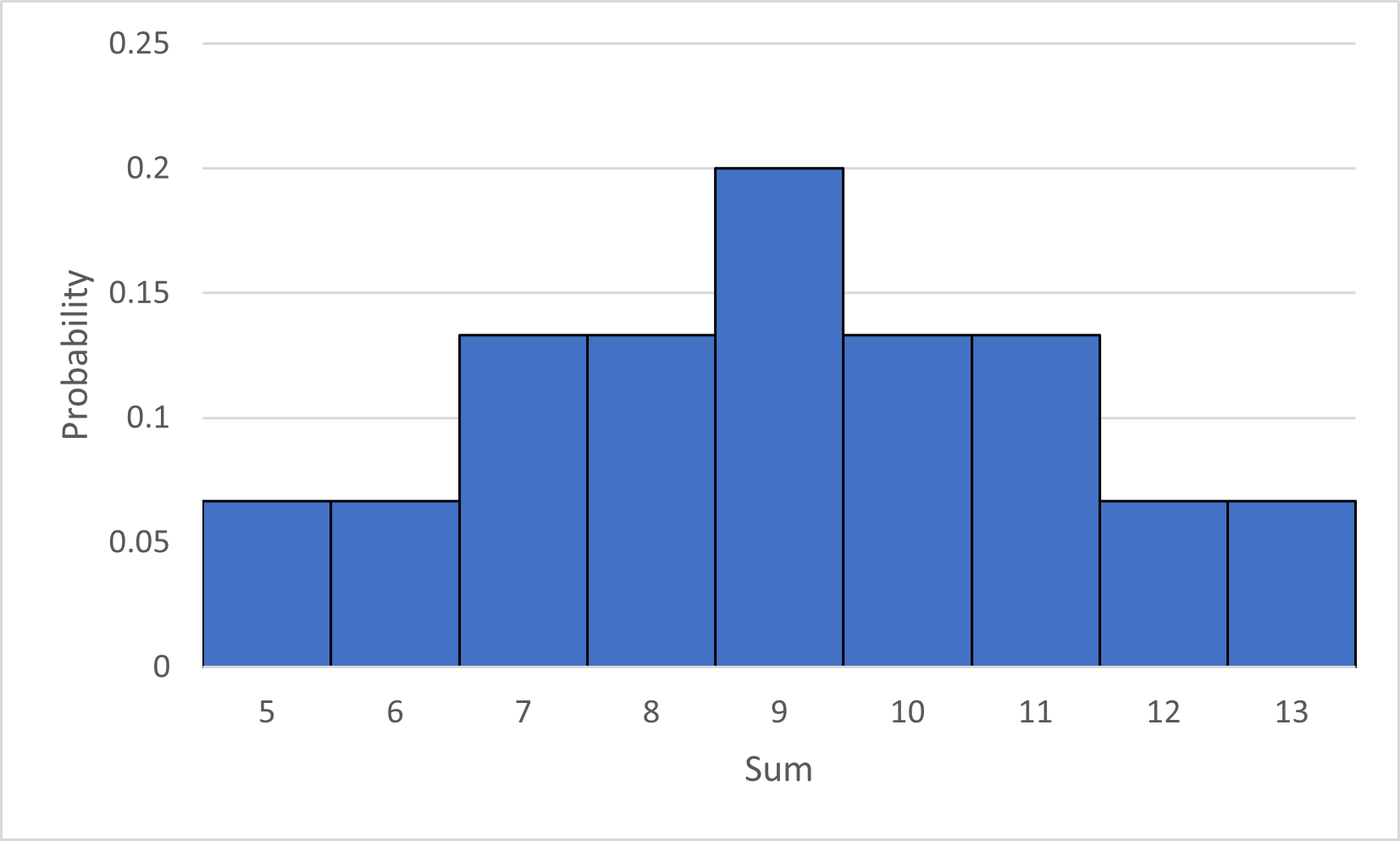
Example 3.1.5. The sum of two cards.
Suppose we take the 2, 3, 4, 5, 6, and 7 of spades from a deck of cards, shuffle these six cards, then add together the values of the top two cards. The outcomes of this experiment are the possible sums: the integers 5 - 13. Below is the probability distribution of this experiment, in table and graph form. (It is possible to calculate the probability of each outcome by hand. Try it yourself for an extra challenge!)
| Sum of card values |
5 |
6 |
7 |
8 |
9 |
10 |
11 |
12 |
13 |
| Probability |
\(\frac{1}{15}\) |
\(\frac{1}{15}\) |
\(\frac{2}{15}\) |
\(\frac{2}{15}\) |
\(\frac{1}{5}\) |
\(\frac{2}{15}\) |
\(\frac{2}{15}\) |
\(\frac{1}{15}\) |
\(\frac{1}{15}\) |
The table allows us to quickly calculate the probability of any event:
The probability that the sum of the cards is either 7 or 13 is
\begin{equation*}
\frac{2}{15} + \frac{1}{15} = \frac{3}{15} = \frac{1}{5} = 0.2,
\end{equation*}
or 20%.
The probability that the sum of the cards is even is
\begin{equation*}
\frac{1}{15} + \frac{2}{15} + \frac{2}{15} + \frac{1}{15} = \frac{6}{15} = \frac{2}{5} = 0.4,
\end{equation*}
or 40%.
The bar graph allows us to more easily see the way the probability is distributed over the possible outcomes. For example, you likely noticed that this probability distribution is symmetric, centered at the outcome 9. Therefore, if we performed this experiment many times, we should expect the most common outcome to be 9 and the average of all the outcomes to be 9. We should also expect that an outcome greater than 11 is less likely than an outcome smaller than 8, since we can see that the area of the bars to the right of 11 is less than the area of the bars to the left of 8.
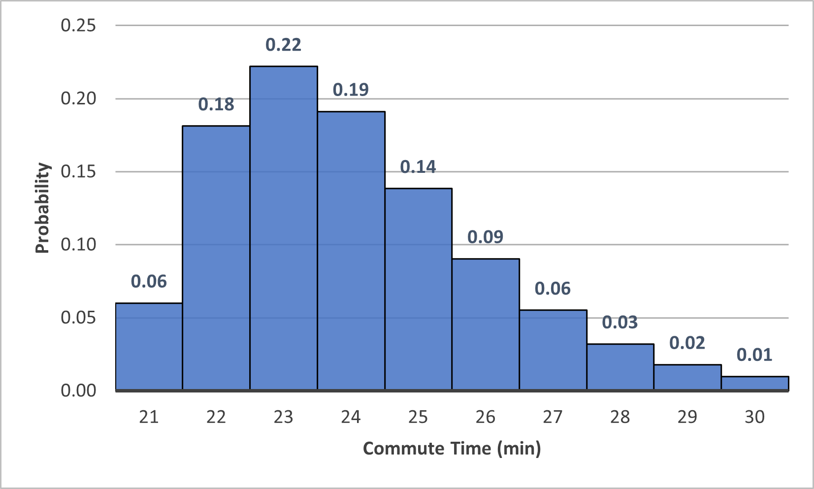
Exploration 3.1.3.
Consider the following probability distribution for the amount of time you spend commuting to work on a given day (rounded to the nearest number of minutes).
What is the probability that your commute takes 27 minutes or longer?
Is it more likely that your commute takes more than 24 minutes or less than 23 minutes?
If asked how long your commute takes, what number of minutes would you say?
Do you think the average number of minutes you take to get to work is less than, greater than, or equal to the number you chose for the previous part? If there is any difference, what do you think causes it?
Solution.
\(0.06+0.03+0.02+0.01 = 0.12\) or 12%
We could compute the probabilities, but looking at the graph it seems clear that there is more area in the bars to the right of 24 minutes than to the left of 23 minutes. So we can confidently say, without any calculations, that it is more likely for your commute to take more than 24 minutes.
This is certainly subjective, but if you had to simplify this to a single number, as people often do, 23 minutes probably makes the most sense. Your commute takes between 22 and 24 minutes the majority (59%) of the time, and it most commonly takes 23 minutes.
Unlike the previous example with the sum of two cards, this probability distribution is not symmetric; it trails off to the right. This means that there is more probability on the right side of the peak. Therefore, it’s most likely that you will tend to take longer than 23 minutes on average. This may be caused by the fact that random occurrences that cause delays are likely to have a more significant impact on your commute than ones that save you time. For example, a bad traffic day would probably cause a longer delay than the amount of time that particularly clear roads would save you.
Exploration 3.1.4.
You may have seen a weather forecast giving the chance of rain over the course of a day in a bar graph that looks something like this:
Is this a probability distribution? Explain why or why not.
Solution.
This graph is not a probability distribution. The horizontal axis lists times of day that it could rain, and it is possible that it could rain across multiple times. Since it could rain at 4:00pm and at 5:00pm, for example, these times cannot be considered the list of outcomes of an experiment. You might also have noticed that the probabilities all together will add up to much more than 100%, which also reflects the fact that it could rain at multiple times throughout the day.