Nathan Wakefield, Christine Kelley, Marla Williams, Michelle Haver, Lawrence Seminario-Romero, Robert Huben, Aurora Marks, Stephanie Prahl, Based upon Active Calculus by Matthew Boelkins
In previous chapters, we have seen that a function’s derivative tells us the rate at which the function is changing. The Fundamental Theorem of Calculus helped us determine the total change of a function over an interval from the function’s rate of change. For instance, an object’s velocity tells us the rate of change of that object’s position. By integrating the velocity over a time interval, we can determine how much the position changes over that time interval. If we know where the object is at the beginning of that interval, we have enough information to predict where it will be at the end of the interval.
In this chapter, we introduce the concept of differential equations. A differential equation is an equation that provides a description of a function’s derivative, which means that it tells us the function’s rate of change. Using this information, we would like to learn as much as possible about the function itself. Ideally we would like to have an algebraic description of the function. Unfortunately, this is too much to ask in some situations, but you are still be able to make accurate approximations. However, for this chapter we will stick to cases in which we can find an explicit solution to a differential equation.
Subsection5.3.1What is a differential equation?
A differential equation is an equation that describes the derivative, or derivatives, of a function that is unknown to us. For instance, the equation
describes the derivative of a function \(y(x)\) that is unknown to us.
Many important examples of differential equations involve quantities that change in time; the independent variable in our discussion will frequently be time \(t\text{.}\) For example, the differential equation
describes an objects position (given by \(s(t)\)) as a function of time.
If we know the velocity and the starting position of a moving object, we will be able to find its position at any later time.
Because differential equations describe the derivative of a function, they give us information about how that function changes. Our goal will be to use this information to predict the value of the function in the future; in this way, differential equations are a type of "crystal ball."
Example5.24.
The position of a moving object is given by the function \(s(t)\text{,}\) where \(s\) is measured in feet and \(t\) in seconds. Assume that the object has velocity given by \(v(t) = 4t + 1\) feet per second.
How much does the position change over the time interval \([0,4]\text{?}\)
Does this give you enough information to determine \(s(4)\text{,}\) the position at time \(t=4\text{?}\) If so, what is \(s(4)\text{?}\) If not, what additional information would you need to know to determine \(s(4)\text{?}\)
Suppose you are told that the object’s initial position \(s(0) = 7\) ft. Determine \(s(2)\text{,}\) the object’s position 2 seconds later.
If we know that \(s(0) = 7\) ft. can we find an equation for \(s(t)\text{?}\)
Hint.
What does the quantity \(\int_0^4 (4t+1)dt\) represent in this problem?
Answer.
36 feet
No, we need to know where the object started.
\(s(2)=17\text{.}\)
\(\displaystyle s(t)=2t^2+t+7\)
Solution.
We can find the total change in the position of the object by integrating the equation for velocity over the interval \([0,4]\text{.}\) That is
Therefore, the position changes by 36 feet over the interval \([0,4]\text{.}\)
Simply knowing how much the position has changed on the interval \([0,4]\) does not tell us where the object is. In order to know where the object is located we must also know where the object started.
We can find the total change in the position of the object by integrating the equation for velocity over the interval \([0,2]\text{.}\) That is
Therefore, the position changes by 10 feet over the interval \([0,2]\text{.}\) Since we know that \(s(0)=7\text{,}\) we can say that \(s(2)=7+10=17\) ft.
Since \(s(0) = 7\) ft, it is reasonable to use \(s(0)\) to "find" the constant \(C\text{.}\) That is, we can say that \(7=2(0)^2+0+C\) which means \(C=7\text{.}\) Therefore, the position of the object at anytime is given by the equation \(s(t)=2t^2+t+7\text{.}\)
Subsection5.3.2Solving a differential equation
A differential equation describes the derivative, or derivatives, of a function that is unknown to us. By a solution to a differential equation, we simply mean a function that satisfies this description.
For instance, the first differential equation we looked at is
which describes an unknown function \(s(t)\text{.}\) We may check that \(s(t) = 2t^2+t\) is a solution because it satisfies this description. Notice that \(s(t) = 2t^2+t+4\) is also a solution.
If we have a candidate for a solution, it is straightforward to check whether it is a solution or not. Before we demonstrate, let’s consider the same issue in a simpler context. Suppose we are given the equation \(2x^2 - 2x = 2x+6\) and asked whether \(x=3\) is a solution. To answer this question, we could rewrite the variable \(x\) in the equation with the symbol \(\Box\text{:}\)
To determine whether \(x=3\) is a solution, we can investigate the value of each side of the equation separately when the value \(3\) is placed in \(\Box\) and see if indeed the two resulting values are equal. Doing so, we observe that
Since \(\frac{dv}{dt}\) and \(1.5 - 0.5v\) agree for all values of \(t\) when \(v = 3-2e^{-0.5t}\text{,}\) we have indeed found a solution to the differential equation.
Which of the following functions are solutions of this differential equation?
\(v(t) = 1.5t - 0.25t^2\text{.}\)
\(v(t) = 3 + 2e^{-0.5t}\text{.}\)
\(v(t) = 3\text{.}\)
\(v(t) = 3 + Ce^{-0.5t}\) where \(C\) is any constant.
Hint.
Calculate \(\frac{dv}{dt}\) and compare that with \(1.5 - 0.5v\) to see if the quantities are equal.
Answer.
\(v(t) = 1.5t - 0.25t^2\) is not a solution to the given DE.
\(v(t) = 3 + 2e^{-0.5t}\) is a solution to the given DE.
\(v(t) = 3\) is a solution to the given DE.
\(v(t) = 3 + Ce^{-0.5t}\) is a solution to the given DE for any choice of \(C\text{.}\)
Solution.
Since \(v(t) = 1.5t - 0.25t^2\text{,}\)\(\frac{dv}{dt} = 1.5 - 0.5t\text{.}\) We observe that for this choice of \(v\text{,}\)\(1.5 - 0.5v = 1.5 - 0.5(1.5t - 0.25t^2) = 1.5 - 0.75t + 0.125t^2 \ne 1.5 - 0.5t = \frac{dv}{dt}\text{,}\) and thus \(v(t) = 1.5t - 0.25t^2\) is not a solution to the given differential equation.
Since \(v(t) = 3 + 2e^{-0.5t}\text{,}\)\(\frac{dv}{dt} = 2e^{-0.5t}(-0.5) = -e^{-0.5t}\text{.}\) Hence, for this choice of \(v\text{,}\)\(1.5 - 0.5v = 1.5 - 0.5(3+2e^{-0.5t}) = 1.5 - 1.5 - e^{-0.5t} = -e^{-0.5t} = \frac{dv}{dt}\text{.}\) Therefore \(v(t) = 3 + 2e^{-0.5t}\) is a solution to the given differential equation.
Since \(v(t) = 3\text{,}\)\(\frac{dv}{dt} = 0\text{.}\) Hence, for this choice of \(v\text{,}\)\(1.5 - 0.5v = 1.5 - 0.5(3) = 1.5 - 1.5 = 0 = \frac{dv}{dt}\text{.}\) Therefore \(v(t) = 3\) is a solution to the given differential equation.
Since \(v(t) = 3 + Ce^{-0.5t}\) (where \(C\) is a constant), \(\frac{dv}{dt} = Ce^{-0.5t}(-0.5) = -0.5C e^{-0.5t}\text{.}\) Hence, for this choice of \(v\text{,}\)\(1.5 - 0.5v = 1.5 - 0.5(3+Ce^{-0.5t}) = 1.5 - 1.5 - 0.5Ce^{-0.5t} = -0.5Ce^{-0.5t} = \frac{dv}{dt}\text{.}\) Therefore \(v(t) = 3 + Ce^{-0.5t}\) is a solution to the given differential equation for any choice of \(C\text{.}\)
This example shows us something interesting. Notice that the differential equation has infinitely many solutions, which are parametrized by the constant \(C\) in \(v(t) = 3+Ce^{-0.5t}\text{.}\) In Figure 5.26, we see the graphs of these solutions for a few values of \(C\text{,}\) as labeled.
Figure5.26.The family of solutions to the differential equation \(\frac{dv}{dt} = 1.5 - 0.5v\text{.}\)
Notice that the value of \(C\) is connected to the initial value of the velocity \(v(0)\text{,}\) since \(v(0) = 3+C\text{.}\) In other words, while the differential equation describes how the velocity changes as a function of the velocity itself, this is not enough information to determine the velocity uniquely: we also need to know the initial velocity. For this reason, differential equations will typically have infinitely many solutions, one corresponding to each initial value. We have seen this phenomenon before: given the velocity of a moving object \(v(t)\text{,}\) we cannot uniquely determine the object’s position function unless we also know its initial position.
If we are given a differential equation and an initial value for the unknown function, we say that we have an initial value problem. For instance,
is an initial value problem. In this problem, we know the value of \(v\) at one time and we know how \(v\) is changing. Consequently, there should be exactly one function \(v\) that satisfies the initial value problem.
This demonstrates the following important general property of initial value problems.
Initial value problems that are “well behaved” have exactly one solution, which exists in some interval around the initial point.
We won’t worry about what “well behaved” means —it is a technical condition that will be satisfied by all the differential equations we consider.
Subsection5.3.3Summary
A differential equation is simply an equation that describes the derivative(s) of an unknown function.
Physical principles, as well as some everyday situations, often describe how a quantity changes, which lead to differential equations.
A solution to a differential equation is a function whose derivatives satisfy the equation’s description. Differential equations typically have infinitely many solutions, parametrized by the initial values.
where \(y\) is the thickness of the ice in centimeters at time \(t\) measured in hours since the ice started forming, and \(k\) is a positive constant. Find \(y\) as a function of \(t\text{.}\)
\(y =\)
2.Setting up a Differential Equation.
If a car goes from 0 to 75 mph in 7 seconds with constant acceleration, what is that acceleration?
\(a =\)\(\mathrm{ft/s^2}\text{.}\)
3.Setting up a Differential Equation.
A cat, walking along the window ledge of a New York apartment, knocks off a flower pot, which falls to the street 230 feet below. How fast is the flower pot traveling when it hits the street? (Give your answer in ft/s and in mi/hr, given that the acceleration due to gravity is \(32 \ \mathrm{ft/s^2}\) and 1 ft/s = 15/22 mi/hr.)
speed in ft/s =
speed in mi/hr =
4.Displacement.
The velocity function is \(v(t) = t^2 - 5 t + 6\) for a particle moving along a line. Find the displacement (net distance covered) of the particle during the time interval \([-3,5]\text{.}\)
displacement =
5.Initial Value Problems.
Use the given information to find the position, velocity, speed, and acceleration at time \(t = 1\text{.}\)
\begin{equation*}
a = 3e^{4t-4}; s = \frac{3}{16 e^{4}}; \; v = \frac{3}{4 e^{4}}
\end{equation*}
when \(t = 0\)
Position \(=\)
Velocity \(=\)
Speed \(=\)
Acceleration \(=\)
6.Initial Velocity.
A projectile fired downward from a height of \(\small{134} ft\) reaches the ground in \(\small{2} s\text{.}\) What is its initial velocity?
Initial Velocity \(ft/s\)
7.Finding the Position Function.
A particle moves along an \(\small{s}\)-axis, use the given information to find the position function of the particle.
A particle moves in a straight line with velocity \(t^{-2} - \frac {1}{9}\) ft/s. Find the total displacement and total distance traveled over the time interval \([1,4]\text{.}\)
Displacement: ft.
Distance: ft.
10.Finding Displacement.
The velocity (in ft/s) of an object moving along a straight line is given by
\begin{equation*}
v(t) = -52 t + 200
\end{equation*}
Find the displacement of the object over the given time intervals.
a) Displacement on \([1, 6]\text{:}\)
ft
s
ft/s
b) Displacement on \([0, 10]\text{:}\)
ft
s
ft/s
11.Finding Displacement from a Graph.
The velocity of an object was measured using a laser radar gun. The following data were collected.
time (sec)
0
1
2
3
4
5
6
7
8
velocity (feet/sec)
-2
-1
-1
-2
-4
0
0
4
2
You decide to plot these velocity data and connect successive data points with lines, as in the following graph. This graph determines a function \(v_{approx}(t)\) that approximates the actual velocity function \(v_{actual}(t)\text{,}\) which is unknown. By connecting data points with lines in the graph you are assuming that velocity is changing at a constant rate over one-second time intervals (or, equivalently, that acceleration is constant over one-second time intervals). This assumption may be incorrect because the actual rate of change of velocity may not be constant over one-second time intervals. However, you decide to use this graph anyway since it seems like a reasonable approximation to the actual velocity.
Graph of approximation to velocity \(y = v_{approx}(t)\)
Using this graph, you can estimate the displacement of the object after \(x\) seconds have elapsed by the value of the function
(A) Using the function \(s(x)\text{,}\) answer the following questions about how far the object traveled. Your answers must include the correct units 14
/webwork2_files/helpFiles/Units.html
.
Displacement after 5 seconds =
Total displacement =
Total distance traveled =
(B) From the graph above, indicate the time interval or union of time intervals where the object is moving forward, backward, and is stationary. Enter your answer using interval notation 15
/webwork2_files/helpFiles/IntervalNotation.html
.
Forward:
Backward:
Stationary:
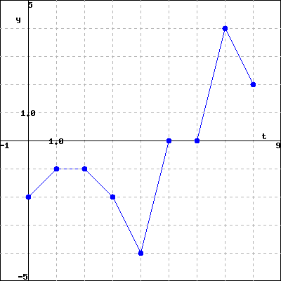
12.Finding Displacement from a Graph.
The velocity of an object was measured using a laser radar gun. The following data were collected.
time (sec)
0
1
2
3
4
5
6
7
8
velocity (feet/sec)
-4
-4
-1
0
0
2
4
2
4
You decide to plot these velocity data and connect successive data points with lines, as in the following graph. This graph determines a function \(v_{approx}(t)\) that approximates the actual velocity function \(v_{actual}(t)\text{,}\) which is unknown. By connecting data points with lines in the graph you are assuming that velocity is changing at a constant rate over one-second time intervals (or, equivalently, that acceleration is constant over one-second time intervals). This assumption may be incorrect because the actual rate of change of velocity may not be constant over one-second time intervals. However, you decide to use this graph anyway since it seems like a reasonable approximation to the actual velocity.
Graph of approximation to velocity \(y = v_{approx}(t)\)
Using this graph, you can estimate the displacement of the object after \(x\) seconds have elapsed by the value of the function
(A) Using the function \(s(x)\text{,}\) answer the following questions about how far the object traveled. Your answers must include the correct units 16
/webwork2_files/helpFiles/Units.html
.
Displacement after 3 seconds =
Total displacement =
Total distance traveled =
(B) From the graph above, indicate the time interval or union of time intervals where the object is moving forward, backward, and is stationary. Enter your answer using interval notation 17