CC Using Derivatives to Identify Extreme Values

🔗

Section 3.1 Using Derivatives to Identify Extreme Values

🔗

Motivating Questions

What are the critical numbers of a function $f$ and how are they connected to identifying the most extreme values the function achieves?
How does the first derivative of a function reveal important information about the behavior of the function, including the function’s extreme values?
How can the second derivative of a function be used to help identify extreme values of the function?

🔗

Supplemental Videos.

🔗

The main topics of this section are also presented in the following videos:

Extreme Values
¹
unl.yuja.com/V/Video?v=7114319&node=34303282&a=120597043&autoplay=1
Derivative Tests
²
unl.yuja.com/V/Video?v=7114321&node=34303287&a=151449745&autoplay=1
Examples
³
unl.yuja.com/V/Video?v=7114320&node=34303227&a=172541093&autoplay=1

🔗

In many different settings, we are interested in knowing where a function achieves its least and greatest values. These can be important in applications – such as identifying a point at which maximum profit or minimum cost occurs – or in theory such as characterizing the behavior of a function or of a family of related functions.

🔗

Consider the simple and familiar example of a parabolic function such as

s (t) = - 16 t^{2} + 32 t + 48

(shown on the left of Figure 3.1 below) that represents the height of an object tossed vertically: its maximum value occurs at the vertex of the parabola and represents the greatest height the object reaches. This maximum value is an especially important point on the graph, the point at which the curve changes from increasing to decreasing.

🔗

Global (Absolute) Maximum and Minimum.

🔗

Given a function

f,

we say that

f (c)

is a global (or absolute) maximum of

f

provided that

f (c) \geq f (x)

for all

x

in the domain of

f .

Similarly, we call

f (c)

a global (or absolute) minimum of

f

whenever

f (c) \leq f (x)

for all

x

in the domain of

f .

🔗

Consider, for example, the graph of

y = g (x)

on the right of Figure 3.1 below. The function

g

has a global maximum of

g (c),

but

g

does not appear to have a global minimum, as the graph of

g

seems to decrease without bound. Note that the point

(c, g (c))

marks a fundamental change in the behavior of

g

g

changes from increasing to decreasing; similar things happen at both

(a, g (a))

and

(b, g (b)),

although these points are not global minima or maxima.

🔗
Figure 3.1. On the left, the graph of $y = s (t),$ where $s (t) = - 16 t^{2} + 24 t + 32$ is a parabola whose vertex is $(\frac{3}{4}, 41);$ on the right, the graph of $y = g (x),$ where $g$ is a function that demonstrates several high and low points.

🔗

Local (Relative) Maximum and Minimum.

🔗

We say that

f (c)

is a local (or relative) maximum of

f

provided that

f (c) \geq f (x)

for all

x

near

c .

Likewise,

f (c)

is called a local (or relative) minimum of

f

whenever

f (c) \leq f (x)

for all

x

near

c .

🔗

For example, returning to the right half of Figure 3.1 above,

g

has a relative minimum of

g (b)

at the point

(b, g (b))

and a relative maximum of

g (a)

(a, g (a)) .

We have already identified the global maximum of

g

g (c);

it can also be considered a relative maximum. Another piece of terminology to be familiar with is that any maximum or minimum may also be called an extreme value of

f .

🔗

We would like to use calculus ideas to identify and classify key function behavior, including the location of relative extrema. Of course, if we are given a graph of a function, it is often straightforward to locate these important behaviors visually. We see this below in Example 3.2.

Example 3.2.

Consider the function

h

given by the graph in Figure 3.3 below. Use the graph to answer each of the following questions.

Figure 3.3. The graph of $y = h (x)$ on the interval $[- 3, 3] .$

Identify all of the values of $c$ for which $h (c)$ is a local maximum of $h .$
Identify all of the values of $c$ for which $h (c)$ is a local minimum of $h .$
Does $h$ have a global maximum on the interval $[- 3, 3] ?$ If so, what is the value of this global maximum?
Does $h$ have a global minimum on the interval $[- 3, 3] ?$ If so, what is its value?
Identify all values of $c$ for which $h^{'} (c) = 0 .$
Identify all values of $c$ for which $h^{'} (c)$ does not exist.
True or false: every relative maximum and minimum of $h$ occurs at a point where $h^{'} (c)$ is either zero or does not exist.
True or false: at every point where $h^{'} (c)$ is zero or does not exist, $h$ has a relative maximum or minimum.

Hint.

Start by looking for $x$ -values where the graph switches from increasing to decreasing. Are there any other points that might work?
Start by looking for $x$ -values where the graph switches from decreasing to increasing. Are there any other points that might work?
Is there a highest point on the graph?
Is there a lowest point on the graph?
Remember that horizontal lines have a slope of $0 .$
Think back to earlier chapters. What characteristics of $h$ or its graph might make it nondifferentiable at a certain point?
Compare your answers to (a) and (b) with those to (e) and (f).
Compare your answers to (a) and (b) with those to (e) and (f).

Answer.

$c = - 2$ and $c = 1 .$
$c = 0 .$
$h (1) = 2 .$
$h (- 3) = - 3 .$
$c = - 2.5$ and $c = 1 .$
$c = - 2,$ $c = 0,$ and $c = 1.5 .$
True.
False.

Solution.

The graph shows that $h (x) \leq - 1 = h (- 2)$ for every $x$ near $- 2$ and $h (x) \leq 2 = h (1)$ for every $x$ near $1 .$ We notice that these are points where $h$ switches from increasing to decreasing. Since there are no other points on the graph where the $y$ -coordinate is larger than everything nearby, it follows that the only local maxima of $h$ on this domain occur at $c = - 2$ and $c = 1 .$
The graph shows that $h (x) \geq - 2 = h (0)$ for every $x$ near $0,$ a point where $h$ switches from decreasing to increasing. However, because we are looking at a restricted domain, on the left we see that $h$ starts out by going up, so $h (x) \geq - 3 = h (- 3)$ for every $x$ near to (and greater than) $- 3 .$ Similarly, on the right we see that $h$ finishes by going down, so $h (x) \geq - 1.25 = h (3)$ for all $x$ near to (and less than) $3 .$ At the very least, then, we can say that the local minima of $h$ on the domain $[- 3, 3]$ are $c = - 3,$ $c = 0,$ and $c = 3 .$

Again, we emphasize that the endpoints of the domain are special. If the graph extended to either side, we could not say with certainty whether the points $(- 3, h (- 3))$ and $(3, h (3))$ are local minima or not. They might be, if the graph changed direction again, but they would not be if the graph followed the existing trend.
The highest point shown on the graph is the point $(1, 2) .$ Since $h$ is continuous on $[- 3, 3],$ we don’t have to worry about any points on the interval being higher and not showing up on the displayed grid. Hence we say the global maximum of $h$ on the interval $[- 3, 3]$ is $2$ and occurs at $x = 1 .$
The lowest point shown on the graph is the point $(- 3, - 3) .$ Again, since $h$ is continuous on $[- 3, 3],$ we don’t have to worry about any points on the interval being lower and not showing up in the window that is displayed. Thus we say the global minimum of $h$ on the interval $[- 3, 3]$ is $- 3$ and occurs at $x = - 3 .$

It is worth noting that this was not a point that we found as a local minimum. The difference is that here we are restricting our focus to the interval that is shown, effectively cutting off the graph at its endpoints. Earlier, when we were looking for relative minima, we made the assumption that the graph of $y = h (x)$ continues outside of the depicted interval by following the trends displayed and continuing downward on both sides.
When looking for points $(c, h (c))$ at which $h^{'} (c) = 0,$ we are looking for points of horizontal tangency. The graph flattens out at $(- 2.5, - 2)$ and $(1, 2),$ but nowhere else
⁴
Note that at $(1.5, 1)$ it looks as though the graph is flat to the right of this point. However, the derivative is undefined here because of the cusp, so this is not a point of horizontal tangency
. Thus $h^{'} (c) = 0$ exactly when $c = - 2.5$ and $c = 1 .$
Recall that $h^{'} (c)$ only exists when all of the following are true:
- $h (c)$ is defined,
- $lim_{x \to c} h (x)$ exists,
- $lim_{x \to c} h (x) = h (c),$ and
- $lim_{a \to 0} \frac{h (c + a) - h (c)}{a}$ exists.
Assuming $h$ is continuous at $c$ (i.e. the first three points hold), the main consequence of the final point is that a corner or a cusp at $(c, h (c))$ makes $h$ nondifferentiable at $c .$
With all this in mind, we can say that $h^{'} (c)$ does not exist at $c = - 2,$ $c = 0,$ or $c = 1.5$ because $h$ has a cusp at these points.
This is true. Every relative extremum of $h$ occurs at a point where $h^{'} (c)$ is either zero or does not exist.
This is false. Some points at which $h^{'} (c)$ is zero or undefined are not relative extrema. In particular, $h^{'} (- 2.5)$ is zero, but the graph is non-decreasing near $(- 2.5, - 2) .$ Similarly, $h^{'} (1.5)$ is undefined, but the graph is non-increasing near $(1.5, 1) .$ Neither of these points is a local maximum or minimum.

🔗

Subsection 3.1.1 Critical Points and the First Derivative Test

🔗
Figure 3.4. From left to right: a function with a relative maximum where its derivative is zero; a function with a relative maximum where its derivative is undefined; a function with neither a maximum nor a minimum at a point where its derivative is zero; a function with a relative minimum where its derivative is zero; and a function with a relative minimum where its derivative is undefined.

🔗

Suppose a function

f

is continuous on an open interval

(a, b) .

f

has a relative maximum at some number

c

in this interval, then

f

must be increasing in some interval just before

c

and decreasing in some interval just after

c .

These intervals could be quite small. Conversely, if

f

is increasing in an interval just before

c

and decreasing in an interval just after

c,

then

f

must have a relative maximum at

c .

The natural analogue holds for relative minima: if

f

has a relative minimum at some number

c

in this interval, then

f

is decreasing in some interval just before

c

and increasing just after

c .

Conversely, if

f

is decreasing in some interval just before

c

and decreasing in an interval just after

c,

then

f

must have a relative minimum at

c .

(See Figure 3.4 above.) There are only two possible ways for these changes in behavior to occur: either

f^{'} (c) = 0

f^{'} (c)

is undefined. Because these values of

c

are so important, we call the point

(c, f (c))

a critical point.

🔗

Critical Point.

🔗

We say that a function

f

has a critical point at

(c, f (c))

provided that

c

is in the domain of

f,

and

f^{'} (c) = 0

f^{'} (c)

is undefined. When

(c, f (c))

is a critical point, we say that

c

is a critical number of the function, or that

f (c)

is a critical value.

🔗

Critical points are the only possible locations where the function

f

may have relative

⁵

Absolute extrema occur only at critical points or at endpoints for functions defined on a fixed domain.

extrema. Note that not every critical point produces a maximum or minimum; in the middle graph of Figure 3.4, the function pictured there has a horizontal tangent line at the noted point, but the function is increasing before and increasing after, so the critical point does not yield a maximum or minimum. Two other such points appeared earlier in Figure 3.3 of Example 3.2.

🔗

The first derivative test summarizes how sign changes in the first derivative (which can only occur at critical numbers) indicate the presence of a local maximum or minimum for a given function.

🔗

First Derivative Test.

🔗

p

is a critical number of a continuous function

f

that is differentiable near

p

(except possibly at

x = p

), then

f

has a relative maximum at

p

if and only if

f^{'}

changes sign from positive to negative at

p,

and

f

has a relative minimum at

p

if and only if

f^{'}

changes sign from negative to positive at

p .

Example 3.5.

Let

f

be a function whose derivative is given by the formula

f^{'} (x) = e^{- 2 x} (3 - x) (x + 1)^{2} .

Determine all critical numbers of

f

and decide whether a relative maximum, relative minimum, or neither occurs at each.

Hint.

When is

f^{'} (x) = 0 ?

What else do you need to look for?

Answer.

- 1

is a critical number that is not a relative extremum.

3

is a local maximum.

Solution.

Since we already have

f^{'} (x)

written in factored form, it is straightforward to find the critical numbers of

f .

Because

f^{'} (x)

is defined for all values of

x,

we need only determine where

f^{'} (x) = 0 .

From the equation

e^{- 2 x} (3 - x) (x + 1)^{2} = 0

and the zero product property

⁶

The zero product property says that if

a b = 0,

where

a

and

b

are expressions representing real numbers (e.g.

a = (3 - x),

where

x

is a real number), then it must be the case that

a = 0

b = 0

(or both).

, it follows that

x = 3

and

x = - 1

are critical numbers of

f .

(There is no value of

x

that makes

e^{- 2 x} = 0 .

)

Next, to apply the first derivative test, we’d like to know the sign of

f^{'} (x)

at inputs near the critical numbers. Because the critical numbers are the only locations at which

f^{'}

can change sign, it follows that the sign of the derivative is the same on each of the intervals created by the critical numbers: for instance, the sign of

f^{'}

must be the same for every

x < - 1 .

What this means is that we can choose (carefully) where to evaluate the derivative in order to ascertain its sign on a given interval. Since

f^{'} (- 1.000001)

and

f^{'} (- 2)

must have the same sign, we may as well evaluate

f^{'} (x)

- 2

to figure out the sign of

f^{'}

for

x < - 1 .

We create a first derivative sign chart (displayed below, with explanation following) to summarize the sign of

f^{'}

on the relevant intervals, along with the corresponding behavior of

f .

Figure 3.6. The first derivative sign chart for a function $f$ whose derivative is given by the formula $f^{'} (x) = e^{- 2 x} (3 - x) (x + 1)^{2} .$

To produce the first derivative sign chart in Figure 3.6, we start by marking the critical numbers

- 1

and

3

on the number line. We then identify the sign of each factor of

f^{'} (x)

at one selected point in each interval. The intervals in this example are

x < - 1,

- 1 < x < 3,

and

x > 3;

we will choose

x = - 2,

x = 0,

and

x = 5

for our selected points. The process with

x = - 2

is laid out below:

For

x < - 1,

we use the value

x = - 2

to determine the sign of

e^{- 2 x},

(3 - x),

and

(x + 1)^{2} .

We note that

e^{- 2 x}

is positive regardless of the value of

x,

(x + 1)^{2}

is positive whenever it is nonzero — which is everywhere within the intervals of interest since we intentionally plucked out the zeros — and that

(3 - x)

is also positive at

x = - 2 .

Hence each of the three terms in

f^{'}

is positive, and we indicate this by writing “

+ + +

” above the interval

x < - 1 .

Taking the product of three positive terms results in a positive value for

f^{'},

so we denote the sign of

f^{'}

by a “

+

” above the appropriate interval in the chart. Finally, since

f^{'}

is positive on that interval, we know that

f

is increasing, so we write “INC” to represent the behavior of

f .

In a similar fashion, we find that

f^{'}

is positive (because

3 - (0) > 0

and the other terms are also still positive) and

f

is increasing on

- 1 < x < 3,

and that

f^{'}

is negative (because

3 - (5) < 0

but the other terms are still positive) and

f

is decreasing for

x > 3 .

Now we look for critical numbers at which

f^{'}

changes sign. In this example,

f^{'}

changes sign only at

x = 3,

from positive to negative, so

f

has a relative maximum at

x = 3 .

Although

f

has a critical number at

x = - 1,

since

f

is increasing both before and after

x = - 1,

f

has neither a minimum nor a maximum at

x = - 1 .

Example 3.7.

Suppose

g

is a function that is continuous for every value of

x \neq 2,

and whose first derivative is

g^{'} (x) = \frac{(x + 4) (x - 1)^{2}}{x - 2} .

Further, assume that it is known that

g

has a vertical asymptote at

x = 2 .

Determine all critical numbers of $g .$
By developing a carefully labeled first derivative sign chart, decide whether $g$ has as a local maximum, local minimum, or neither at each critical number.
Does $g$ have a global maximum? Does $g$ have a global minimum? Justify your claims.
What is the value of $lim_{x \to \infty} g^{'} (x) ?$ What does the value of this limit tell you about the long-term behavior of $g ?$
Sketch a possible graph of $y = g (x) .$

Hint.

For which $x$ is $g^{'} (x) = 0 ?$
Note that $(x - 1)^{2}$ is positive for all $x \neq 1 .$
Use your first derivative sign chart from (b).
Try expanding the numerator before evaluating the limit.
Think carefully about the information from the sign chart found in (b). Your answers to part (c) and (d) should also support your graph.

Answer.

$x = - 4$ or $x = 1 .$
$g$ has a local maximum at $x = - 4$ and neither a max nor min at $x = 1 .$
$g$ does not have a global minimum; it is unclear (at this point in our work) if $g$ increases without bound, so we can’t say for certain whether or not $g$ has a global maximum.
$lim_{x \to \infty} g^{'} (x) = \infty .$
A possible graph of $g$ is the following.

Solution.

Since $g^{'} (x) = \frac{(x + 4) (x - 1)^{2}}{x - 2},$ we see that $g^{'} (x) = 0$ implies that $x = - 4$ or $x = 1 .$ Although $x = 2$ makes $g^{'}$ undefined, we are told that $g$ has a vertical asymptote at $x = 2 .$ So $x = 2$ is not in the domain of $g,$ and hence is technically not a critical number of $g .$ Nonetheless, we place $x = 2$ on our first derivative sign chart since the vertical asymptote is a location at which $g^{'}$ may change sign.
The first derivative sign chart shows that:
- $g^{'} (x) > 0$ for $x < - 4,$
- $g^{'} (x) < 0$ for $- 4 < x < 1,$
- $g^{'} (x) < 0$ for $1 < x < 2,$ and
- $g^{'} (x) > 0$ for $x > 2 .$
By the first derivative test, $g$ has a local maximum at $x = - 4$ and neither a max nor min at $x = 1 .$ As these are the only two critical numbers, these are the only two locations for possible extrema. (Note: although $g$ changes from decreasing to increasing at $x = 2,$ this is due to a vertical asymptote, and $g$ does not have a minimum there.)
Because $g$ is decreasing as $x \to 2^{-}$ (where $g$ has a vertical asymptote), $g$ does not have a global minimum. For $x > 2,$ $g$ is always increasing, which suggests that $g$ does not have a global maximum (though we do not know for sure that $g$ increases without bound; this is explored in part (d)).
We observe that

$\begin{aligned} lim_{x \to \infty} g^{'} (x) = & lim_{x \to \infty} \frac{(x + 4) (x - 1)^{2}}{x - 2} \\ = & lim_{x \to \infty} \frac{x^{3} + 2 x^{2} - 7 x + 4}{x - 2} \cdot \frac{\frac{1}{x}}{\frac{1}{x}} \\ = & lim_{x \to \infty} \frac{x^{2} + 2 x - 7 + \frac{4}{x}}{1 - \frac{2}{x}} \\ = & \infty \end{aligned}$

Since $g^{'} (x) \to \infty$ as $x \to \infty,$ this tells us that $g$ increases without bound as $x \to \infty .$
From all of our work above, we know that $g$ has a local maximum at $x = - 4,$ a horizontal tangent line with neither a max nor min at $x = 1,$ and a vertical asymptote at $x = 2,$ plus $g$ and $g^{'}$ both increase without bound as $x \to \infty .$ Thus, a possible graph of $y = g (x)$ is the following.

🔗

Subsection 3.1.2 The Second Derivative Test

🔗

Recall that the second derivative of a function tells us several important things about the behavior of the function itself. For instance, if

f^{″}

is positive on an interval, then we know that on that interval

f^{'}

is increasing and, consequently, that

f

is concave up. Hence throughout that interval the tangent line to

y = f (x)

lies below the curve at every point. At a point where

f^{'} (p) = 0,

the sign of the second derivative determines whether

f

has a local minimum or local maximum at the critical number

p .

🔗
Figure 3.8. Four possible graphs of a function $f$ with a horizontal tangent line at a critical point.

🔗

In Figure 3.8 above, we see the four possibilities for a function

f

that has a critical number

p

at which

f^{'} (p) = 0,

provided

f^{″} (p)

is not zero on an interval including

p

(except possibly at

p

). On either side of the critical number,

f^{″}

can be either positive or negative, and hence

f

can be either concave up or concave down. In the first two graphs,

f

does not change concavity at

p

and

f

has either a local minimum or local maximum in those situations. In particular, if

f^{'} (p) = 0

and

f^{″} (p) < 0,

then

f

is concave down at

p

with a horizontal tangent line, so

f

has a local maximum there. This fact, along with the corresponding statement for when

f^{″} (p)

is positive, is the substance of the second derivative test.

🔗

Second Derivative Test.

🔗

p

is a critical number of a continuous function

f

such that

f^{'} (p) = 0

and

f^{″} (p) \neq 0,

then

f

has a relative maximum at

p

if and only if

f^{″} (p) < 0,

and

f

has a relative minimum at

p

if and only if

f^{″} (p) > 0 .

🔗

In the event that

f^{″} (p) = 0,

the second derivative test is inconclusive. That is, the test doesn’t provide us any information. This is because if

f^{″} (p) = 0,

it is possible that

f

has a local minimum, local maximum, or neither.

⁷

Consider the functions

f (x) = x^{4},

g (x) = - x^{4},

and

h (x) = x^{3}

at the critical point

p = 0 .

🔗

Just as a first derivative sign chart reveals all of the increasing and decreasing behavior of a function, we can construct a second derivative sign chart that demonstrates all of the important information involving concavity.

Example 3.9.

Let

f

be a function whose first derivative is

f^{'} (x) = 3 x^{4} - 9 x^{2} .

Construct both first and second derivative sign charts for

f;

fully discuss where

f

is increasing, decreasing, concave up, and concave down; identify all relative extreme values; and sketch a possible graph of

f .

Solution.

Since we know

f^{'} (x) = 3 x^{4} - 9 x^{2},

we can find the critical numbers of

f

by solving

3 x^{4} - 9 x^{2} = 0 .

Factoring, we observe that

0 = 3 x^{2} (x^{2} - 3) = 3 x^{2} (x + \sqrt{3}) (x - \sqrt{3}),

so that

x = 0, \pm \sqrt{3}

are the three critical numbers of

f .

The first derivative sign chart for

f

is given below in Figure 3.10.

Figure 3.10. The first derivative sign chart for $f$ when $f^{'} (x) = 3 x^{4} - 9 x^{2} = 3 x^{2} (x^{2} - 3) .$

We see that

f

is increasing on the intervals

(- \infty, - \sqrt{3})

and

(\sqrt{3}, \infty),

and

f

is decreasing on

(- \sqrt{3}, 0)

and

(0, \sqrt{3}) .

By the first derivative test, this information tells us that

f

has a local maximum at

x = - \sqrt{3}

and a local minimum at

x = \sqrt{3} .

Although

f

also has a critical number at

x = 0,

neither a maximum nor minimum occurs there since

f^{'}

does not change sign at

x = 0 .

Next, we move on to investigate concavity. Differentiating

f^{'} (x) = 3 x^{4} - 9 x^{2},

we see that

f^{″} (x) = 12 x^{3} - 18 x .

Since we are interested in knowing the intervals on which

f^{″}

is positive and negative, we first find where

f^{″} (x) = 0 .

Observe that

0 = 12 x^{3} - 18 x = 12 x (x^{2} - \frac{3}{2}) = 12 x (x + \sqrt{\frac{3}{2}}) (x - \sqrt{\frac{3}{2}}) .

This equation has solutions

x = 0, \pm \sqrt{\frac{3}{2}} .

Building a sign chart for

f^{″}

in the exact same way we do for

f^{'},

we see the result shown below in Figure 3.11.

Figure 3.11. The second derivative sign chart for $f$ when $f^{″} (x) = 12 x^{3} - 18 x = 12 x^{2} (x^{2} - \sqrt{\frac{3}{2}}) .$

Therefore

f

is concave down on the intervals

(- \infty, - \sqrt{\frac{3}{2}})

and

(0, \sqrt{\frac{3}{2}}),

and concave up on

(- \sqrt{\frac{3}{2}}, 0)

and

(\sqrt{\frac{3}{2}}, \infty) .

Putting all of this information together, we now see a complete and accurate possible graph of

f

in Figure 3.12.

Figure 3.12. A possible graph of the function $f$ in Example 3.9.

The point

A = (- \sqrt{3}, f (- \sqrt{3}))

is a local maximum, because

f

is increasing prior to

A

and decreasing after; similarly, the point

E = (\sqrt{3}, f (\sqrt{3})

is a local minimum. Note, too, that

f

is concave down at

A

and concave up at

E,

which is consistent both with our second derivative sign chart and the second derivative test. At points

B

and

D,

concavity changes, as we saw in the results of the second derivative sign chart in Figure 3.11. Finally, at point

C,

f

has a critical point with a horizontal tangent line, but neither a maximum nor a minimum occurs there, since

f

is decreasing both before and after

C .

It is also the case that concavity changes at

C .

While we completely understand where

f

is increasing and decreasing, where

f

is concave up and concave down, and where

f

has relative extrema, we do not know any specific information about the

y

-coordinates of points on the curve. For instance, while we know that

f

has a local maximum at

x = - \sqrt{3},

we don’t know the value of that maximum because we do not know

f (- \sqrt{3}) .

Any vertical translation of our sketch of

f

in Figure 3.12 would satisfy the given criteria for

f .

🔗

Points

B,

C,

and

D

in Figure 3.12 are locations at which the concavity of

f

changes. We give a special name to any such point.

🔗

Inflection Point.

🔗

Let

f

be a continuous function. If

p

is a point in the domain of

f

at which

f

changes concavity, then we say that

(p, f (p))

is an inflection point (or point of inflection) of

f .

🔗

Just as we look for locations where

f

changes from increasing to decreasing at points where

f^{'} (p) = 0

f^{'} (p)

is undefined, so too we find where

f^{″} (p) = 0

f^{″} (p)

is undefined to see if there are points of inflection at these locations.

🔗

At this point in our study, it is important to remind ourselves of the big picture that derivatives help to paint: the sign of the first derivative

f^{'}

tells us whether the function

f

is increasing or decreasing, while the sign of the second derivative

f^{″}

tells us how the function

f

is increasing or decreasing.

Example 3.13.

Suppose that

g

is a function whose second derivative,

g^{″},

is given by the graph in Figure 3.14 below.

Figure 3.14. The graph of $y = g^{″} (x) .$

Find the $x$ -coordinates of all points of inflection of $g .$
Fully describe the concavity of $g$ by making an appropriate sign chart.
Suppose you are given that $g^{'} (- 1.67857351) = 0 .$ Is there a local maximum, local minimum, or neither (for the function $g$ ) at this critical number of $g,$ or is it impossible to say? Why?
Assuming that $g^{″} (x)$ is a polynomial (and that all important behavior of $g^{″}$ is seen in the graph above), what degree polynomial do you think $g (x)$ is? Why?

Hint.

What must be true of $g^{″} (x)$ at a point of inflection?
Use the given graph to decide where $g^{″}$ is positive and negative.
What does the second derivative test say?
Can you guess a formula for $g^{″} (x)$ based on its graph?

Answer.

$x = - 1$ is an inflection point of $g .$
$g$ is concave up for $x < - 1,$ concave down for $- 1 < x < 2,$ and concave down for $x > 2 .$
$g$ has a local minimum at $x = - 1.67857351 .$
$g$ is a degree 5 polynomial.

Solution.

Based on the given graph of $g^{″},$ the only point at which $g^{″}$ changes sign is $x = - 1,$ so this is the only inflection point of $g .$
Note that $g^{″} (x) > 0$ for $x < - 1,$ $g^{″} (x) < 0$ for $- 1 < x < 2,$ and $g^{″} (x) < 0$ for $x > 2 .$ This tells us that $g$ is concave up for $x < - 1,$ concave down for $- 1 < x < 2,$ and concave down for $x > 2 .$
Given that $g^{'} (- 1.67857351) = 0,$ we know that $g$ has a horizontal tangent line at this critical number. Additionally, the graph of $y = g^{″} (x)$ shows that $g^{″} (- 1.67857351) > 0,$ so we infer that $g$ is concave up at $x$ -values near $- 1.67857351 .$ The second derivative test allows us to conclude that $g$ has a local minimum at $x = - 1.67857351 .$
As seen in the given graph, since $g^{″}$ has a simple zero at $x = - 1$ and a repeated zero at $x = 2,$ it appears that $g^{″}$ is a degree 3 polynomial. If so, then $g^{'}$ is a degree 4 polynomial, and $g$ is a degree 5 polynomial.

🔗

As we will see in more detail in the following section, derivatives also help us to understand families of functions that differ only by changing one or more parameters. For instance, we might be interested in understanding the behavior of all functions of the form

f (x) = a (x - h)^{2} + k

where

a,

h,

and

k

are parameters. Each parameter has considerable impact on how the graph appears.

Example 3.15.

Consider the family of functions given by

h (x) = x^{2} + \cos (k x),

where

k

is an arbitrary positive real number.

Use a graphing utility to sketch the graph of $y = h (x)$ for several different $k$ -values, including $k = 1, 3, 5, 10 .$ What is the smallest value of $k$ at which you think you can see (just by looking at the graph) at least one inflection point on the graph of $h ?$
Explain why the graph of $h$ has no inflection points if $k \leq \sqrt{2},$ but infinitely many inflection points if $k > \sqrt{2} .$
Explain why, no matter the value of $k,$ $h$ can only have finitely many critical numbers.

Hint.

Be sure to try some values between 1.5 and 2.
Treat $k$ as an arbitrary constant in computing $h^{'} (x)$ and $h^{″} (x) .$
What is the largest value of $k \sin (k x) ?$ How many times can $y = k \sin (k x)$ intersect the line $y = 2 x ?$

Answer.

In the graph below, $h (x) = x^{2} + \cos (3 x)$ is given in dark blue, while $h (x) = x^{2} + \cos (1.6 x)$ is shown in light blue.
If $\frac{2}{k^{2}} > 1,$ then the equation $\cos (k x) = \frac{2}{k^{2}}$ has no solution. Hence, whenever $k^{2} < 2,$ or $k < \sqrt{2} \approx 1.414,$ it follows that the equation $\cos (k x) = \frac{2}{k^{2}}$ has no solutions $x,$ which means that $h^{″} (x)$ is never zero (indeed, for these $k$ -values, $h^{″} (x)$ is always positive so that $h$ is always concave up). On the other hand, if $k \geq \sqrt{2}$ then $\frac{2}{k^{2}} \leq 1,$ which guarantees that $\cos (k x) = \frac{2}{k^{2}}$ has infinitely many solutions due to the periodicity of the cosine function. At each such point, $h^{″} (x)$ changes sign if and only if $k > \sqrt{2} .$ (In the case where $k = \sqrt{2},$ the function $h^{″}$ has infinitely many zeros but is always non-negative.) Therefore $h$ has infinitely many inflection points whenever $k > \sqrt{2},$ and no inflection points otherwise.
To see why $h$ can only have a finite number of critical numbers regardless of the value of $k,$ consider the equation

$0 = h^{'} (x),$

which implies that $2 x = k \sin (k x) .$ Since $- 1 \leq \sin (k x) \leq 1,$ we know that $- k \leq k \sin (k x) \leq k .$ Once $| x |$ is sufficiently large, we are guaranteed that $| 2 x | > k,$ which means that for large values of $x,$ the graphs of $y = 2 x$ and $y = k \sin (k x)$ cannot intersect. Moreover, for relatively small values of $x,$ the functions $2 x$ and $k \sin (k x)$ can only intersect finitely many times since $k \sin (k x)$ only oscillates a finite number of times on a fixed interval. This is why $h$ can only have a finite number of critical numbers, regardless of the value of $k .$

Solution.

In the graph below, $h (x) = x^{2} + \cos (3 x)$ is given in dark blue, while $h (x) = x^{2} + \cos (1.6 x)$ is shown in light blue.

Close inspection of the light blue graph reveals some subtle changes in concavity around $x \approx \pm 0.5 .$ For values smaller than $1.6,$ it is very hard to visually detect any inflection points in $h (x) .$
Treating $k$ as an arbitrary constant, we first observe that $h^{'} (x) = 2 x - k \sin (k x) .$ Again treating $k$ as a constant and differentiating, we find

$h^{″} (x) = 2 - k^{2} \cos (k x) .$

We seek the values of $x$ at which $h^{″} (x) = 0$ and $h^{″}$ changes sign. Setting $h^{″} (x) = 0$ and rearranging the resulting equation, we now seek $x$ such that

$k^{2} \cos (k x) = 2,$

or

$\cos (k x) = \frac{2}{k^{2}} .$

Now, remember that $k$ is an arbitrary positive constant and recall that $- 1 \leq \cos (θ) \leq 1$ for all input values $θ .$ If $\frac{2}{k^{2}} > 1,$ then the equation $\cos (k x) = \frac{2}{k^{2}}$ has no solution. Hence, whenever $k^{2} < 2,$ or $k < \sqrt{2} \approx 1.414,$ it follows that the equation $\cos (k x) = \frac{2}{k^{2}}$ has no solutions, which means that $h^{″} (x)$ is never zero (indeed, for these $k$ -values, $h^{″} (x)$ is always positive so that $h$ is always concave up). On the other hand, if $k \geq \sqrt{2}$ then $\frac{2}{k^{2}} \leq 1,$ which guarantees that $\cos (k x) = \frac{2}{k^{2}}$ has infinitely many solutions due to the periodicity of the cosine function. At each such point, $h^{″} (x)$ changes sign if and only if $k > \sqrt{2} .$ (In the case where $k = \sqrt{2},$ the function $h^{″}$ has infinitely many zeros but is always non-negative.) Therefore $h$ has infinitely many inflection points whenever $k > \sqrt{2},$ and no inflection points otherwise.
To see why $h$ can only have a finite number of critical numbers regardless of the value of $k,$ recall that $h^{'} (x) = 2 x - k \sin (k x)$ and consider the equation

$0 = h^{'} (x),$

which then implies that $2 x = k \sin (k x) .$ Since $- 1 \leq \sin (k x) \leq 1,$ we know that $- k \leq k \sin (k x) \leq k .$ Once $| x |$ is sufficiently large, we are guaranteed that $| 2 x | > k,$ which means that for large values of $x,$ the graphs of $y = 2 x$ and $y = k \sin (k x)$ cannot intersect. Moreover, for relatively small values of $x,$ the functions $2 x$ and $k \sin (k x)$ can only intersect finitely many times since $k \sin (k x)$ only oscillates a finite number of times on a finite interval. This is why $h$ can only have a finite number of critical numbers, regardless of the value of $k .$

🔗

Subsection 3.1.3 Summary

🔗

The critical numbers of a continuous function $f$ are the values of $p$ for which $f^{'} (p) = 0$ or $f^{'} (p)$ does not exist. These values are important because they identify horizontal tangent lines or corner points on the graph, which are the only possible locations at which a local maximum or local minimum can occur.
Given a differentiable function $f :$ whenever $f^{'}$ is positive, $f$ is increasing; whenever $f^{'}$ is negative, $f$ is decreasing. The first derivative test tells us that at any point where $f$ changes from increasing to decreasing, $f$ has a local maximum, while conversely at any point where $f$ changes from decreasing to increasing $f$ has a local minimum.
Given a twice differentiable function $f,$ if we have a horizontal tangent line at $x = p$ and $f^{″} (p)$ is nonzero, the sign of $f^{″}$ tells us the concavity of $f$ and hence whether $f$ has a maximum or minimum at $x = p .$ In particular, if $f^{'} (p) = 0$ and $f^{″} (p) < 0,$ then $f$ is concave down at $p$ and $f$ has a local maximum there, while if $f^{'} (p) = 0$ and $f^{″} (p) > 0,$ then $f$ has a local minimum at $p .$ If both $f^{'} (p) = 0$ and $f^{″} (p) = 0,$ then the second derivative test does not tell us whether $f$ has a local extremum at $p$ or not.

🔗

Exercises 3.1.4 Exercises

🔗

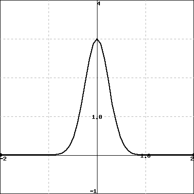
1. Finding critical points and inflection points.

🔗

Use a graph below of

f (x) = 3 e^{- 8 x^{2}}

to estimate the

x

-values of any critical points and inflection points of

f (x) .

🔗

critical points (enter as a comma-separated list):

x =

🔗

inflection points (enter as a comma-separated list):

x =

🔗

Next, use derivatives to find the

x

-values of any critical points and inflection points exactly.

🔗

critical points (enter as a comma-separated list):

x =

🔗

inflection points (enter as a comma-separated list):

x =

🔗

2. Finding inflection points.

🔗

Find the inflection points of

f (x) = 2 x^{4} + 10 x^{3} - 18 x^{2} + 12 .

(Give your answers as a comma separated list, e.g., 3,-2.)

🔗

inflection points =

🔗

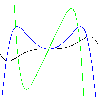
3. Matching graphs of $f, f^{'}, f^{″}$ .

🔗

The following shows graphs of three functions, A (in black), B (in blue), and C (in green). If these are the graphs of three functions

f,

f^{'},

and

f^{″},

identify which is which.

🔗

(Click on the graph to get a larger version.)

🔗

(For each enter A, B or C).

🔗

f =

;

f^{'} =

;

f^{″} =

🔗

4. Using a derivative graph to analyze a function.

🔗

This problem concerns a function about which the following information is known:

$f$ is a differentiable function defined at every real number $x$
$f (0) = - \frac{1}{2}$
$y = f^{'} (x)$ has its graph given at center in Figure 3.16

Figure 3.16. At center, a graph of $y = f^{'} (x);$ at left, axes for plotting $y = f (x);$ at right, axes for plotting $y = f^{″} (x) .$

🔗

Construct a first derivative sign chart for $f .$ Clearly identify all critical numbers of $f,$ where $f$ is increasing and decreasing, and where $f$ has local extrema.
On the right-hand axes, sketch an approximate graph of $y = f^{″} (x) .$
Construct a second derivative sign chart for $f .$ Clearly identify where $f$ is concave up and concave down, as well as all inflection points.
On the left-hand axes, sketch a possible graph of $y = f (x) .$

🔗

5. Using derivative tests.

🔗

Suppose that

g

is a differentiable function and

g^{'} (2) = 0 .

In addition, suppose that on

1 < x < 2

and

2 < x < 3

it is known that

g^{'} (x)

is positive.

Does $g$ have a local maximum, local minimum, or neither at $x = 2 ?$ Why?
Suppose that $g^{″} (x)$ exists for every $x$ such that $1 < x < 3 .$ Reasoning graphically, describe the behavior of $g^{″} (x)$ for $x$ -values near $2 .$
Besides being a critical number of $g,$ what is special about the value $x = 2$ in terms of the behavior of the graph of $g ?$

🔗

6. Using a derivative graph to analyze a function.

🔗

Suppose that

h

is a differentiable function whose first derivative is given by the graph in Figure 3.17.

🔗

How many real number solutions can the equation $h (x) = 0$ have? Why?
If $h (x) = 0$ has two distinct real solutions, what can you say about the signs of the two solutions? Why?
Assume that $lim_{x \to \infty} h^{'} (x) = 3,$ as appears to be indicated in Figure 3.17. How will the graph of $y = h (x)$ appear as $x \to \infty ?$ Why?
Describe the concavity of $y = h (x)$ as fully as you can from the provided information.

Figure 3.17. The graph of $y = h^{'} (x) .$

🔗

7. Applying derivative tests.

🔗

Let

p

be a function whose second derivative is

p^{″} (x) = (x + 1) (x - 2) e^{- x} .

Construct a second derivative sign chart for $p$ and determine all inflection points of $p .$
Suppose you also know that $x = \frac{\sqrt{5} - 1}{2}$ is a critical number of $p .$ Does $p$ have a local minimum, local maximum, or neither at $x = \frac{\sqrt{5} - 1}{2} ?$ Why?
If the point $(2, \frac{12}{e^{2}})$ lies on the graph of $y = p (x)$ and $p^{'} (2) = - \frac{5}{e^{2}},$ find the equation of the tangent line to $y = p (x)$ at the point where $x = 2 .$ Does the tangent line lie above the curve, below the curve, or neither at this value? Why?

Prev Top Next

Section 3.1 Using Derivatives to Identify Extreme Values

Motivating Questions

Supplemental Videos.

Global (Absolute) Maximum and Minimum.

Local (Relative) Maximum and Minimum.

Example 3.2.

Subsection 3.1.1 Critical Points and the First Derivative Test

Critical Point.

First Derivative Test.

Example 3.5.

Example 3.7.

Subsection 3.1.2 The Second Derivative Test

Second Derivative Test.

Example 3.9.

Inflection Point.

Example 3.13.

Example 3.15.

Subsection 3.1.3 Summary

Exercises 3.1.4 Exercises

1. Finding critical points and inflection points.

2. Finding inflection points.

3. Matching graphs of f,f′,f″.

4. Using a derivative graph to analyze a function.

5. Using derivative tests.

6. Using a derivative graph to analyze a function.

7. Applying derivative tests.

3. Matching graphs of $f, f^{'}, f^{″}$ .