\(\newcommand{\dollar}{\$} \DeclareMathOperator{\erf}{erf} \DeclareMathOperator{\arctanh}{arctanh} \newcommand{\lt}{<} \newcommand{\gt}{>} \newcommand{\amp}{&} \)

Section3.7Parametric Equations

Motivating Questions
  • What types of equations can be used to describe motion in multiple dimensions as a function of time?

  • How can we calculate instantaneous rates of change for such equations?

  • How can we derive the equations of lines tangent to such equations?

Up to this point, we have been representing a graph by a single equation involving two variables such as \(x\) and \(y\text{.}\) However, some items are not really well described by such equations. In this section, you will study situations in which it is useful to introduce a third variable to represent a curve in the plane. This process is commonly called parameterization and is the basis for our study of parametric curves.

SubsectionParametric Equations

Consider the path of an object that is propelled into the air at an angle of \(45^{\circ}\text{.}\) In a physics class, you might learn that this object would follow a parabolic path. That is,

\begin{equation*} y=-\frac{x^2}{72}+x \end{equation*}

However, this equation does not tell the whole story. While the equation does tell you where the object has been, it does not tell you when the object was at a given point \((x, y)\) on the path. To determine this time, you can introduce a third variable \(t\text{,}\) called a parameter. It is possible to write both \(x\) and \(y\) as functions of \(t\) to obtain the parametric equations

\begin{align*} x(t) \amp= 24 \sqrt{2}t\\ y(t) \amp =-16t^2+24\sqrt{2}t \end{align*}

The parametric equations are graphed in Figure3.69 below. Using the parametric equations, we can state properties such as: at time \(t = 0\text{,}\) the object is at the point \((0, 0)\) and at time \(t = 1\text{,}\) the object is at the point \((24 \sqrt{2},24\sqrt{2}-16)\text{.}\)

Figure3.69A plot of the parametric equations \(x(t)= 24 \sqrt{2}t\text{,}\) \(y(t) =-16t^2+24\sqrt{2}t\text{.}\) Notice that when \(t=\frac{3\sqrt{2}}{4}\text{,}\) \(x=36\) and \(y=18\) (you can get these values by plugging \(t=\frac{3\sqrt{2}}{4}\) into the equations for \(x\) and \(y\)).
Example3.70

Suppose the position of an object is given by the parametric equations

\begin{align*} x(t) \amp= 24 \sqrt{2}t\\ y(t) \amp =-16t^2+24\sqrt{2}t. \end{align*}

After \(t=3\) seconds, what is the position of the object if the origin represents the initial position?

Hint

Try plugging \(t=3\) into each equation.

Answer

After \(3\) seconds the object is located at \((24 \sqrt{2}3,144-72 \sqrt{2}).\)

Solution

By plugging \(t=3\) into each of the equations for \(x(t)\) and \(y(t)\) we see that

\begin{align*} x(3) \amp= 24 \sqrt{2}(3)\\ y(3) \amp =-16(3)^2+24\sqrt{2}(3) \end{align*}

Therefore, after \(3\) seconds the object is located at \((24 \sqrt{2}3,144-72 \sqrt{2}).\)

With these examples in hand we are now in a position to formally define parametric equations.

Parametric Equations

Parametric equations are equations that specify the values of \(x\) and \(y\) in terms of a third variable \(t\) called a parameter. We often represent parametric curves in the form

\begin{align*} x(t) \amp= f(t)\\ y(t) \amp =g(t). \end{align*}

where \(f\) and \(g\) are functions and the parameter \(t\) varies over some interval \(a \lt t \lt b\text{.}\) When no interval is specified we assume that \(t\) accepts all real values.

SubsectionGraphing Parametric Equations

Graphs of curves sketched from parametric equations can have very interesting shapes, as exemplified in Figure3.71. In this section we will cover some methods to sketch parametric curves.

Figure3.71Parametric equations can give some very interesting graphs.

One of the most effective ways to sketch a parametric curve is to create a table of values by choosing various values of \(t\) and computing both \(x(t)\) and \(y(t)\text{.}\) The following example demonstrates this procedure.

Example3.72

Sketch the curve given by the parametric equations

\begin{align*} x(t) \amp= t^2-4\\ y(t) \amp = \frac{t}{2}. \end{align*}
Hint

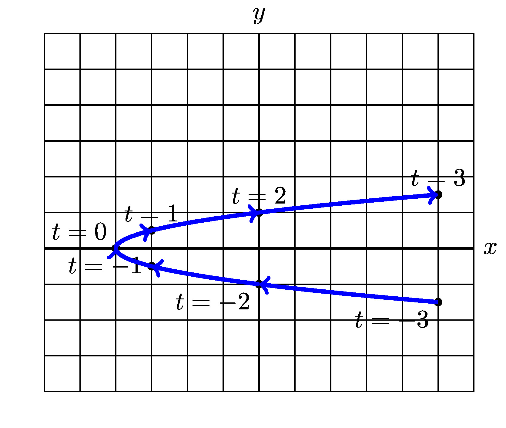
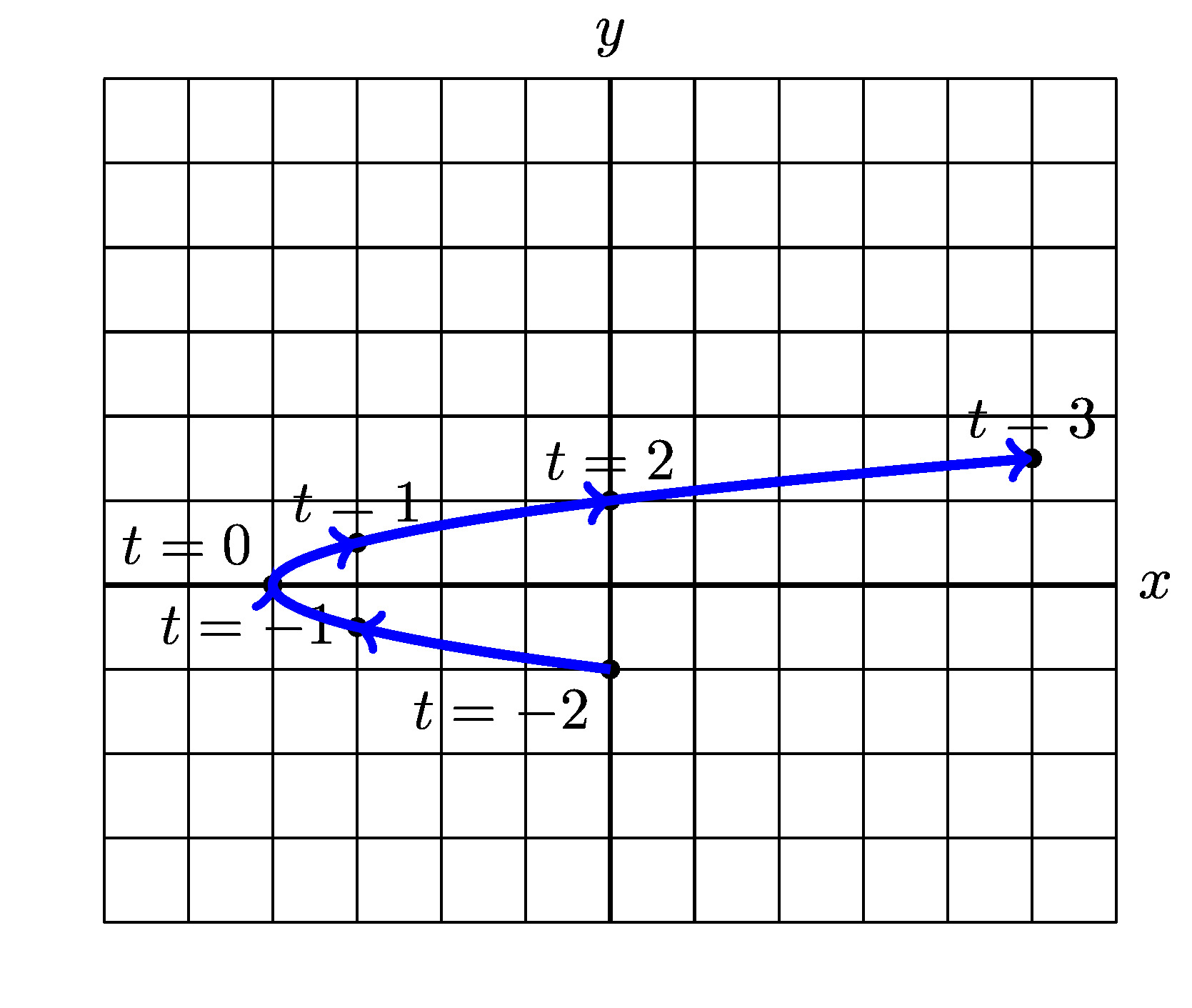
A reasonable first step is to cerate a table of values for \(t=-2,-1,0,1,2,3\text{.}\) Why these values of \(t\text{?}\) Choosing "good" values of \(t\) is not always a straight forward task and in general you must choose values that give you a "reasonable" picture of the curve. You also might wonder how many values of \(t\) are appropriate. Again, the answer is enough values that you can be reasonably confident you have captured the shape of the curve. So what does this mean? Often it helps to choose a few positive and negative values close to zero, calculate these values, plot the points, and then determine if you need more values to give your curve a clear shape.

Answer

We get the following graph by starting at \(t=3\)

Figure3.73Plot of the parametric equations \(x(t)=t^2-4\) and \(y(t)=\frac{t}{2}\) for \(-3 \lt t \lt 3\text{.}\)
Solution

We begin by creating a table of values (For more details on how we chose these value see the hint).

t x(t) y(t)
-2 0 -1
-1 -3 -\frac{1}{2}
0 -4 0
1 -3 \frac{1}{2}
2 0 1
3 5 \frac{3}{2}
Table3.74Table of values for the parametric equations \(x(t)=t^2-4\) and \(y(t)=\frac{t}{2}\)
We plot these values on a coordinate plane and then connect the values with appropriate curves as in Figure3.75. It is often helpful to place arrows on the curve to indicate how the curve changes as \(t\) increases.

Figure3.75Plot of the parametric equations \(x(t)=t^2-4\) and \(y(t)=\frac{t}{2}\) for \(-2 \lt t \lt 3\text{.}\)

You may notice in Figure3.75 that the curve seems to start abruptly at \(t=-2\text{.}\) In fact, this is just an artifact of our starting our table of values at \(t=-2\text{.}\) If we instead started our table at \(t=-3\) then we would get a slightly different image, Figure3.73.

Figure3.76Plot of the parametric equations \(x(t)=t^2-4\) and \(y(t)=\frac{t}{2}\) for \(-3 \lt t \lt 3\text{.}\)

In addition to the method of plotting points, many graphing software programs can effectively plot parametric curves. For convenience, one usch utility based on GeoGebra is included in Figure3.77.

Figure3.77GeoGebra app for plotting parametric equations.
Example3.78

Describe the motion of the particle whose coordinates at time t are expressed with the parametric equations: \(x = \cos(t)\) and \(y = \sin(t)\text{.}\)

Solution

Since \((\cos(t))^2 + (\sin(t))^2 = 1\text{,}\) we have \(x^2 + y^2 = 1\text{.}\) That is, at any time \(t\) the particle is at a point \((x, y)\) on the unit circle \(x^2 + y^2 = 1\text{.}\) We plot points at different times to see how the particle moves on the circle. The particle completes one full trip counterclockwise around the circle every \(2\pi\) units of time. Notice how the \(x\)-coordinate goes back and forth from \(-1\) to \(1\) while the \(y\)-coordinate goes up and down from \(-1\) to \(1\text{.}\) The two motions combine to trace out a circle.

t x y
0 1 0
\(\frac{\pi}{2}\) 0 1
\(\pi\) -1 0
\(\frac{3\pi}{2}\) 0 -1
\(2\pi\) 1 0
Table3.79Table of values for the parametric equations \(x = \cos(t)\) and \(y = \sin(t)\text{.}\)

Figure3.80Plot of the parametric equations \(x = \cos(t)\) and \(y = \sin(t)\text{.}\)

The first thing we note is that \((\cos(3t))^2 + (\sin(3t))^2 = 1\) and so we still have the fact that, at any time \(t\) the particle is at a point \((x, y)\) on the unit circle \(x^2 + y^2 = 1\text{.}\) So, what effect is the \(3\) in \(x = \cos(3t)\) and \(y = \sin(3t)\) having? Consider the following table of values:

t x y
0 1 0
\(\frac{\pi}{6}\) 0 1
\(\frac{\pi}{3}\) -1 0
\(\frac{\pi}{2}\) 0 -1
\(\frac{2\pi}{3}\) 1 0
Table3.81Table of values for the parametric equations \(x = \cos(3t)\) and \(y = \sin(3t)\text{.}\)
In other words, the motion of the particle described by \(x = \cos(3t)\) and \(y = \sin(3t)\) is nearly identical to the motion of a particle described by \(x = \cos(t)\) and \(y = \sin(t)\) except that the particle described by \(x = \cos(3t)\) and \(y = \sin(3t)\) is moving three times as fast. The motion of the particule is displayed by the graph in Figure3.82.
Figure3.82Plot of the parametric equations \(x = \cos(3t)\) and \(y = \sin(3t)\text{.}\)

SubsectionMotion in a Straight Line and Derivatives

Suppose an object moves with constant speed along a straight line through the point \((x_0, y_0)\text{.}\) Recall that they key to motion in a straight line is that the rate of change is constant. In other words, both the \(x\) and \(y\)-coordinates have a constant rate of change. For convenience, let \(a = \frac{dx}{dt}\) and \(b = \frac{dy}{dt}\) be the rate of change in the \(x\) and \(y\) directions, respectively. Then at time \(t\) the object has coordinates \(x = x_0 + at\text{,}\) \(y = y_0 + bt\text{.}\) Notice that \(a\) represents the change in \(x\) in one unit of time, and \(b\) represents the change in \(y\) in one unit of time (see Figure3.83). Thus the line has slope \(m = \frac{b}{a}\text{.}\) Therefore, the parametric equations for motion in a straight line are given by \(x = x_0 + at\text{,}\) \(y = y_0 + bt\text{.}\)

Figure3.83Plot of the parametric equations \(x = \cos(3t)\) and \(y = \sin(3t)\text{.}\)

Now that we have developed the notion of motion in a straight line for parametric equations we can discuss tangent lines for parametric equations.

Parametric Equations for the Tangent Line

An object moving along a line through the point \((x_0, y_0)\text{,}\) with \(\frac{dx}{dt} = a\) and \(\frac{dy}{dt} = b\text{,}\) has parametric equations

\begin{equation*} x = x_0 + at \mbox{, } y = y_0 + bt. \end{equation*}

The slope of the line is \(m = \frac{b}{a}\text{.}\)

Example3.84

Find the tangent line at the point \((1, 2)\) to the curve defined by the parametric equations \(x = t^3\text{,}\) \(y = 2t\text{.}\)

Hint

Try finding the tangent line at the point for each equation separately.

Answer

the tangent line has parametric equations

\begin{equation*} x = 1 + 3t\mbox{, } y = 2 + 2t. \end{equation*}
Solution

At time \(t = 1\) the particle is at the point \((1, 2)\text{.}\) The velocity in the \(x\)-direction at time \(t\) is \(v_x = \frac{dx}{dt} = 3t^2\text{,}\) and the velocity in the \(y\)-direction is \(v_y = \frac{dy}{dt} = 2\text{.}\) So at \(t = 1\) the velocity in the \(x\)-direction is 3 and the velocity in the \(y\)-direction is \(2\text{.}\) Thus the tangent line has parametric equations

\begin{equation*} x = 1 + 3t\mbox{, } y = 2 + 2t. \end{equation*}

With the notion of a tangent line in hand we are in the position to be able to talk about the speed and velocity of an object whose position is given by parametric equations. In general, given an object traveling in the \(xy\)-plane we can break its movement into two pieces. Movement in the "\(x\)-direction" and movement in the "\(y\)-direction." We can also talk about rate-of-change in the "\(x\)-direction" (\(\frac{dx}{dt}\)) and rate-of-change in the "\(y\)-direction" (\(\frac{dy}{dt}\)). If we think of these rates of change as vectors then we can use the Pythagorean theorem to talk about the instantaneous speed \(v\) , see Figure3.85.

Figure3.85Calculation of instantaneous speed based on individual directional component rates of change using Pythagorean theorem.
Using this idea we have the following definition.
Instantaneous Speed

The instantaneous speed of a moving object is defined to be

\begin{equation*} v=\sqrt{\left(\dfrac{dx}{dt} \right)^2+\left(\dfrac{dy}{dt} \right)^2} \end{equation*}

The quantity \(v_x = \frac{dx}{dt}\) is the instantaneous velocity in the \(x\)-direction; \(v_y = \frac{dy}{dt}\) is the instantaneous velocity in the \(y\)-direction. The velocity vector \(\mathbf{v}\) is written

\begin{equation*} \mathbf{v}=v_x \mathbf{i}+v_y\mathbf{j}. \end{equation*}

Example3.86

A particle moves along a curve in the \(xy\)-plane with \(x(t) = 2t + e^t\) and \(y(t) = 3t -4\text{,}\) where \(t\) is time. Find the velocity vector and speed of the particle when \(t = 1\text{.}\)

Hint

Use the formula above after finding the derivative of each equation.

Answer

The speed at \(t = 1\) is

\begin{equation*} v=\sqrt{(2+e)^2+3^2} \approx 5.591\text{.} \end{equation*}
Solution

Differentiating gives \(\frac{dx}{dt} = 2 + e^t\text{,}\) \(\frac{dy}{dt} = 3\text{.}\) When \(t = 1\) we have \(v_x = 2 + e\text{,}\) \(v_y = 3\text{.}\) So the velocity vector is

\begin{equation*} \mathbf{v}=(2+e)\mathbf{i}+3\mathbf{j} \end{equation*}

The speed at \(t = 1\) is

\begin{equation*} v=\sqrt{(2+e)^2+3^2} \approx 5.591\text{.} \end{equation*}

We now formally define the slope of the tangent line to a parametric curve and concavity of a parametric curve.

Slope of Tangent Line to Parametric Curves
\begin{equation*} \dfrac{dy}{dx}=\dfrac{\dfrac{dy}{dt}}{\dfrac{dx}{dt}} \end{equation*}
Concavity of Parametric Curves
\begin{equation*} \dfrac{d^2y}{dx^2}=\dfrac{\dfrac{d}{dt} \left(\dfrac{dy}{dx}\right)}{\dfrac{dx}{dt}} \end{equation*}

Example3.87

A particle moves in the \(xy\)-plane so that its position at time \(t\) is given by \(x = \sin(2t)\text{,}\) \(y = -\cos(2t)\) for \(0 \leq t \lt 2\pi\text{.}\)

  1. At what time does the particle first touch the \(x\)-axis? What is the speed of the particle at that time?
  2. Is the particle ever at rest?
Hint

Recall the \(x\)-axis is where \(y=0\text{.}\) Use the above equation for the speed. If the particle is at rest, think about what the value of the velocity is.

Answer
  1. The particle touches the \(x\)-axis when \(t=\frac{\pi}{4}\text{.}\) At this point, the speed of the particle is
    \begin{equation*} 2\text{.} \end{equation*}
  2. The particle is never at rest.
Solution
  1. The particle touches the \(x\)-axis when \(y=0\text{,}\) that is when \(\cos(2t)=0\text{.}\) This occurs when \(t=\frac{\pi}{4}\text{.}\) At this point, the speed of the particle is given by
    \begin{equation*} \sqrt{4\cos^2(\frac{\pi}{2})+4\sin^2(\frac{\pi}{2})}=2\text{.} \end{equation*}
  2. Since \(\sqrt{4\cos^2(2t)+4\sin^2(2t)}=2\text{,}\) the particle is never at rest.

SubsectionExercises