\(\newcommand{\dollar}{\$} \DeclareMathOperator{\erf}{erf} \DeclareMathOperator{\arctanh}{arctanh} \newcommand{\lt}{<} \newcommand{\gt}{>} \newcommand{\amp}{&} \)

Section2.8Derivatives of Hyperbolic Functions

Motivating Questions
  • What type of function describes the behavior of a line hanging between two poles?

  • What are the properties of a function that can be used to describe the behavior of a line between two poles?

  • What is the derivative of a function that can be used to describe the behavior of a line between two poles?

There is an important class of functions that show up in many real-life situations: the so-called hyperbolic functions. Hyperbolic functions can be used to describe the shape of electrical lines freely hanging between two poles or any idealized hanging chain or cable supported only at its ends and hanging under its own weight. Hyperbolic functions can also be used to describe the path of a spacecraft performing a gravitational slingshot maneuver.

Figure2.95Freely-hanging electric power cables can form a catenary.

SubsectionThe Hyperbolic Trigonometric Functions

There are two fundamental hyperbolic trigonometric functions, the hyperbolic sine (\(\sinh\)) and hyperbolic cosine (\(\cosh\)). These functions are defined in terms of the functions \(e^x\) and \(e^{-x}\text{.}\) Graphs of the hyperbolic sine and hyperbolic cosine are given below in Figure2.96.

Hyperbolic Functions
\begin{equation*} \sinh(x)=\frac{e^x-e^{-x}}{2} \hskip 1cm \cosh(x) = \frac{e^x+e^{-x}}{2} \end{equation*}

Figure2.96On the left, the graphs of \(y=\frac12e^x\) (in red), \(y=-\frac12e^{-x}\) (in blue), and \(y=\sinh(x)\) (in black). On the right, the graphs of \(y=\frac12e^x\) (in red), \(y=\frac12e^{-x}\) (in blue), and \(y=\cosh(x)\) (in black).
Example2.97

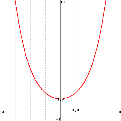
A cable hanging between two supports will form the shape of a hyperbolic cosine. In particular, the formula

\begin{equation*} y = \frac{T}{w}\cosh\left(\frac{wx}{T}\right), \end{equation*}

where \(T\) is the tension at its lowest point and \(w\) is the weight of the cable per unit length, will yield the total cable sag when evaluated at \(x=0\text{.}\) We can calculate the total sag in a powerline hanging between two poles spaced 400 feet apart where the mass per unit length is \(50\) lb/ft and the tension at the lowest point is \(2025\) lbs. Specifically, the total sag is given by

\begin{equation*} y = \frac{2025 \mbox{ lb}}{50 \mbox{ lb/ft}}\cosh\left(\frac{50\times 0}{2025}\right)=40.5 \mbox{ ft}. \end{equation*}

In addition to the hyperbolic sine and cosine, there is also a hyperbolic tangent function which is defined as you might expect.

Hyperbolic Tangent
\begin{equation*} \tanh(x)=\frac{\sinh(x)}{\cosh(x)}=\frac{e^x-e^{-x}}{e^x+e^{-x}} \end{equation*}

SubsectionIdentities and Properties

Similar to the usual trigonometric functions, the hyperbolic trigonometric functions have several important properties. While we will not take the time to directly show these properties are valid, we do encourage the reader to confirm these properties by using the formulas and by inspecting the graphs in Figure2.96 above.

Properties of Hyperbolic Functions
  • \(\cosh(0) = 1\text{;}\)
  • \(\sinh(0) = 0\text{;}\)
  • \(\cosh(-x) = \cosh(x)\text{;}\)
  • \(\sinh(-x) = -\sinh(x)\text{.}\)

It is also useful to discuss the long-run behavior of the hyperbolic trigonometric functions. Again, inspection of Figure2.96 above suggests that as \(x\rightarrow\infty\text{,}\) the graph of \(\cosh(x)\) resembles the graph of \(\frac12e^x\text{.}\) Similarly, it appears that as \(x\rightarrow-\infty\text{,}\) the graph of \(\cosh(x)\) resembles the graph of \(\frac12e^{-x}\text{.}\) This behavior is further explained by using the formulas for \(\cosh(x)\) and \(\sinh(x)\) and the facts that \(e^{-x}\rightarrow0\) as \(x\rightarrow\infty\text{,}\) and \(e^{x}\rightarrow0\) as \(x\rightarrow-\infty\text{.}\)

Recall that the trig functions were defined on the unit circle, giving us the Pythagorean identity: if we set \(x = \cos(\theta)\) and \(y=\sin(\theta)\text{,}\) then the point \((x,y)\) lies on the unit circle, and we have

\begin{equation*} \cos^2(\theta) + \sin^2(\theta) = 1\text{ because }x^2+y^2 = 1\text{.} \end{equation*}

In fact, an analogous identity holds for the hyperbolic trigonometric functions.

A Hyperbolic Identity
\begin{equation*} \cosh^2(\theta) - \sinh^2(\theta) = 1 \end{equation*}

This identity shows us how the hyperbolic functions got their name. Suppose \((x,y)\) is a point in the plane, and \(x = \cosh\theta\) and \(y=\sinh\theta\) for some \(\theta\text{.}\) Then the point \((x,y)\) lies on the hyperbola \(x^2-y^2 = 1\text{.}\)

SubsectionDerivatives of Hyperbolic Functions

We now proceed to calculate the derivatives of each of the hyperbolic functions.

Example2.98

Calculate the derivatives

  1. \(\frac{d}{dx}[\cosh(x)]\)
  2. \(\frac{d}{dx}[\sinh(x)]\)
  3. \(\frac{d}{dx}[\tanh(x)]\)
Hint

Recall that \(\frac{d}{dx}[e^x]=e^x\text{,}\) \(\sinh(x)=\frac{e^x-e^{-x}}{2}\text{,}\) \(\cosh(x) = \frac{e^x+e^{-x}}{2}\text{,}\) and \(\tanh(x)=\frac{\sinh(x)}{\cosh(x)}=\frac{e^x-e^{-x}}{e^x+e^{-x}} \text{.}\)

Answer
  1. \begin{equation*} \frac{d}{dx}[\cosh(x)] =\sinh(x)\text{.} \end{equation*}
  2. \begin{equation*} \frac{d}{dx}[\sinh(x)] = \cosh(x)\text{.} \end{equation*}
  3. \begin{equation*} \frac{d}{dx}[\tanh(x)] =\frac{1}{\cosh^2(x)}\text{.} \end{equation*}
Solution
  1. \begin{equation*} \frac{d}{dx}[\cosh(x)] = \frac{d}{dx}\left[\frac{e^x+e^{-x}}{2}\right]=\frac{e^x-e^{-x}}{2}=\sinh(x)\text{.} \end{equation*}
  2. \begin{equation*} \frac{d}{dx}[\sinh(x)] = \frac{d}{dx}\left[\frac{e^x-e^{-x}}{2}\right]=\frac{e^x+e^{-x}}{2}=\cosh(x)\text{.} \end{equation*}
  3. \begin{equation*} \frac{d}{dx}[\tanh(x)] = \frac{d}{dx}\left[\frac{\sinh(x)}{\cosh(x)}\right]=\frac{(\cosh(x))^2-(\sinh(x))^2}{(\cosh(x))^2}=\frac{1}{\cosh^2(x)}\text{.} \end{equation*}

Derivatives of Hyperbolic Trigonometric Functions
  • \(\frac{d}{dx}[\cosh(x)]=\sinh(x)\text{.}\)
  • \(\frac{d}{dx}[\sinh(x)]=\cosh(x)\text{.}\)
  • \(\frac{d}{dx}[\tanh(x)]=\frac{1}{\cosh^2(x)}\text{.}\)

SubsectionApplications of Hyperbolic Trigonometry

A company wishes to build a suspension bridge that stretches between the basketball arena and the baseball stadium on the other side of the railway lines in a particular city. The center part of the bridge will be suspended between two concrete pillars 280 feet apart and 80 feet high. The cable holding the bridge is to be exactly 30 feet above the railway tracks in the middle of the bridge, i.e. it sags exactly 50 feet.

In 1691, Gottfried Leibniz and Christian Huygens determined that any cable hanging under the force of gravity must have the shape of the graph of

\begin{equation*} y(x) = a \cosh\left( \frac x a \right) + b. \end{equation*}

This shape is known as a catenary. The parameter \(a\) is the ratio of cable tension to cable density. The only use of the parameter \(b\) is to provide a vertical shift, if needed.

We can ask two important questions. First, what values must \(a\) and \(b\) have in order for the catenary to fit the constraints provided by the placement of the concrete pillars and the low point of the cable?

In order to find \(a\) and \(b\) we need to solve two separate equations. We know that \(y(0)=30\) to ensure we have sufficient clearance above the railway tracks. We also know that \(y(140)=80\) since the cable attaches to a 80 foot tall pillar 140 feet from the lowest point (center). Therefore we have

\begin{equation*} 30=a \cosh\left( \frac 0 a \right) + b\text{,} \end{equation*}
\begin{equation*} 80=a \cosh\left( \frac{140}{a} \right) + b\text{.} \end{equation*}

Since \(\cosh(0)=1\) we can simplify the first equation to \(30=a+b\text{.}\) Substituting this equation into the second equation yields \(80=a \cosh\left( \frac{140}{a} \right) +30-a\text{.}\) Now, by graphing the function \(y=x \cosh\left( \frac{140}{x} \right) +30-x\) and the line \(y=80\) and then graphically searching for the point of intersection (as in Figure2.99 below), we see that \(80=a \cosh\left( \frac{140}{a} \right) +30-a\) when \(a \approx 203.82\text{.}\)

Figure2.99Solving \(80=a \cosh\left( \frac{140}{a} \right) +30-a\text{.}\)

Using the value of \(a \approx 203.82\) together with \(30=a+b\) we have \(b=-173.82\text{.}\) Therefore, the height of the bridge can be modeled by the equation

\begin{equation*} h(x)=203.82 \cosh\left(\frac{x}{203.82}\right) - 173.82\text{.} \end{equation*}

SubsectionSummary

  • Hyperbolic functions are useful in modeling the shape of a cable hanging between two poles.

  • The hyperbolic functions are defined in terms of elementary exponential functions:

    \begin{equation*} \sinh(x)=\frac{e^x-e^{-x}}2, \ \ \cosh(x)=\frac{e^x+e^{-x}}2, \ \text{and} \end{equation*}
    \begin{equation*} \tanh(x)=\frac{\sinh(x)}{\cosh(x)}=\frac{e^x-e^{-x}}{e^x+e^{-x}}\text{.} \end{equation*}
  • Hyperbolic sine and hyperbolic cosine satisfy an identity similar to the Pythagorean identity: \(\cosh^2(x)-\sinh^2(x)=1\) for any real number \(x\text{.}\)

  • The derivatives of the hyperbolic functions are also reminiscent of the regular trigonometric derivatives:

    \begin{equation*} \frac{d}{dx}[\sinh(x)]=\cosh(x), \ \ \frac{d}{dx}[\cosh(x)]=\sinh(x), \ \text{and} \end{equation*}
    \begin{equation*} \frac{d}{dx}[\tanh(x)]=\frac1{\cosh^2(x)}\text{.} \end{equation*}

SubsectionExercises