Nathan Wakefield, Christine Kelley, Marla Williams, Michelle Haver, Lawrence Seminario-Romero, Robert Huben, Aurora Marks, Stephanie Prahl, Based upon Active Calculus by Matthew Boelkins
What is the formula for the general tangent line approximation to a differentiable function \(y = f(x)\) at the point \((a,f(a))\text{?}\)
What is the principle of local linearity and what is the local linearization of a differentiable function \(f\) at a point \((a,f(a))\text{?}\)
How does knowing just the tangent line approximation tell us information about the behavior of the original function itself near the point of approximation? How does knowing the second derivative’s value at this point provide us additional knowledge of the original function’s behavior?
Supplemental Videos.
The main topics of this section are also presented in the following videos:
Among all functions, linear functions are simplest. One of the powerful consequences of a function \(y = f(x)\) being differentiable at a point \((a,f(a))\) is that up close the function \(y = f(x)\) is locally linear and looks like its tangent line at that point. In certain circumstances, this allows us to approximate the original function \(f\) with a simpler function \(L\) that is linear: this can be advantageous when we have limited information about \(f\) or when \(f\) is computationally or algebraically complicated. We will explore all of these situations in what follows.
It is essential to recall that when \(f\) is differentiable at \(x = a\text{,}\) the value of \(f'(a)\) provides the slope of the tangent line to \(y = f(x)\) at the point \((a,f(a))\text{.}\) If we know both a point on the line and the slope of the line we can find the equation of the tangent line and write the equation in point-slope form. 40
Recall that a line with slope \(m\) that passes through \((x_0,y_0)\) has equation \(y - y_0 = m(x - x_0)\text{,}\) and this is the point-slope form of the equation.
Example2.100.
Consider the function \(g(x) = -x^2+3x+2\text{.}\)
Use the limit definition of the derivative to compute a formula for \(g'(x)\text{.}\) Check your work using the derivative rules that have been developed throughout this chapter.
Determine the slope of the tangent line to the graph of \(y = g(x)\) at the value \(x = 2\text{.}\)
Compute \(g(2)\text{.}\)
Find an equation for the tangent line to the graph of \(y = g(x)\) at the point \((2,g(2))\text{.}\) Write your result in point-slope form.
Sketch an accurate, labeled graph of \(y = g(x)\) on the interval \(-1\le x\le4\text{.}\) On the same axes, sketch its tangent line at the point \((2,g(2))\text{.}\)
Hint.
Recall the limit definition of the derivative from Chapter 1.
How does the slope of the tangent line relate to the value of the derivative?
Use the given formula for \(g\text{.}\)
Use your answers to (b) and (c).
\(g\) is quadratic, so its graph is a parabola (opening downward).
Answer.
\(g'(x)=-2x+3\text{.}\)
\(g'(2)=-1\text{.}\)
\(g(2)=4\text{.}\)
\(y-4=-1(x-2)\text{.}\)
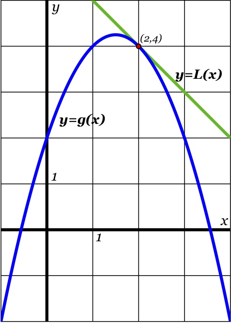
Figure2.101.The graph of \(y=g(x)\) along with its tangent line \(L\) at the point \((2,4)\text{,}\) where \(g(x)=-x^2+3x+2\text{.}\)
Solution.
Since the limit definition of the derivative says that
Figure2.102.The graph of \(y=g(x)\) along with its tangent line \(L\) at the point \((2,4)\text{,}\) where \(g(x)=-x^2+3x+2\text{.}\)
Subsection2.9.1The Tangent Line
Given a function \(f\) that is differentiable at \(x = a\text{,}\) we know that we can determine the slope of the tangent line to \(y = f(x)\) at \((a,f(a))\) by computing \(f'(a)\text{.}\)
The Tangent Line.
The equation of the resulting tangent line is given in point-slope form by
\begin{equation*}
y - f(a) = f'(a)(x-a) \text{.}
\end{equation*}
Warning2.103.
Note: there is a major difference between \(f(a)\) and \(f(x)\) in this context. The former is a constant that results from using the given fixed value of \(a\text{,}\) while the latter is the general expression for the rule that defines the function. The same is true for \(f'(a)\) and \(f'(x)\text{:}\) we must carefully distinguish between these expressions. Each time we find the tangent line, we need to evaluate the function and its derivative at a fixed \(a\)-value.
In Figure 2.104 below, we see the graph of a function \(f\) and its tangent line at the point \((a,f(a))\text{.}\) Notice how when we zoom in we see the local linearity of \(f\) more clearly highlighted. The function and its tangent line are nearly indistinguishable up close. Local linearity can also be seen dynamically in the java applet at http://gvsu.edu/s/6J 41
gvsu.edu/s/6J
.
Figure2.104.The graph of a function \(y = f(x)\) and its tangent line at the point \((a,f(a))\text{:}\) at left, from a distance, and at right, up close. If we let \(L(x)=f'(a)(x-a)+f(a)\) denote the tangent line function, then we observe in the right image that for \(x\) near \(a\text{,}\)\(f(x) \approx L(x)\text{.}\)
Subsection2.9.2The Local Linearization
A slight change in perspective and notation will enable us to be more precise in discussing how the tangent line approximates \(f(x)\) near \(x = a\text{.}\) By solving for \(y\text{,}\) we can write the equation for the tangent line as
\begin{equation*}
y = f'(a)(x-a) + f(a)\text{.}
\end{equation*}
This line is itself a function of \(x\text{.}\) Replacing the variable \(y\) with the expression \(L(x)\text{,}\) we have the following.
the local linearization of \(f\) at the point \((a,f(a))\).
In this notation, \(L(x)\) is nothing more than a "new name" for the tangent line. As we saw above, for \(x\) close to \(a\text{,}\)\(f(x) \approx L(x)\text{.}\) For this reason, \(L(x)\) is also called the tangent line approximation to \(f\) at \((a,f(a))\).
Example2.105.
Suppose that all we know about a function \(f\) is that its tangent line approximation at the point \((1,3)\) is given by \(L(x) = 3 - 2(x-1)\text{.}\) To estimate a value of \(f(x)\) for \(x\) near \(1\text{,}\) such as \(f(1.2)\text{,}\) we can use the fact that \(f(1.2) \approx L(1.2)\text{.}\) Hence
Example2.106.Error in a Tangent Line Approximation.
Consider the function \(p(t)=\ln(t)\text{.}\)
Find the local linearization, \(L(t)\text{,}\) of \(p\) at \(t=1\text{.}\)
Use the tangent line approximation from (a) to estimate the value of \(\ln(1.01)\text{.}\)
Use the tangent line approximation from (a) to estimate the value of \(\ln(1.3)\text{.}\)
The error of an approximation is the difference between the true value and the estimated value. In particular, given a function \(f\) and its local linearization \(L(x)\) at \((a,f(a))\text{,}\) we say the error of the tangent line approximation is
Of the two estimates you found in (b) and (c), which do you expect to be more accurate? Why? Check your guess by calculating and comparing \(E(1.01)\) and \(E(1.3)\text{.}\)
Hint.
Start by finding \(\frac{d}{dt}[\ln(t)]\text{.}\)
By construction of \(L(t)\text{,}\) we know that \(p(1.01)\approx L(1.01)\text{.}\)
Remember that \(p(1.3)\approx L(1.3)\text{.}\)
The approximation should be best close to \(t=1\text{.}\) Note \(E(1)=0\) since \(p(1)=L(1)\text{.}\)
Answer.
\(L(t)=t-1\text{.}\)
\(\ln(1.01)\approx0.01\text{.}\)
\(\ln(1.3)\approx0.3\text{.}\)
We expect \(|E(1.3)|>|E(1.01)|\text{.}\) Indeed, \(E(1.01)=\ln(1.01)-0.01\approx-0.00005\text{,}\) whereas \(E(1.3)=\ln(1.3)-0.3\approx-0.0376\text{.}\)
Solution.
We start by computing \(p'(t)\text{,}\) and then evaluating \(p(1)\) and \(p'(1)\text{.}\) Since \(p(t)=\ln(t)\text{,}\) the derivative is \(p'(t)=\frac1t\text{.}\) Furthermore, we have \(p(1)=\ln(1)=0\) and \(p'(1)=\frac11=1\text{.}\) Thus, the local linearization of \(p(t)=\ln(t)\) at the point \((1,0)\) is
Since we can use the tangent line approximation for \(p\) at \((1,0)\) to estimate output values of \(p\) at nearby points, it follows that \(p(1.01)\approx L(1.01)\text{.}\) Thus we have
Since we can use the tangent line approximation for \(p\) at \((1,0)\) to estimate output values of \(p\) at nearby points, it follows that \(p(1.3)\approx L(1.3)\text{.}\) Thus we have
Since \(1.3\) is farther away from the point of tangency \((t=1)\) than \(1.01\) is, we expect the estimate to be better for \(1.01\text{.}\) We confirm this by computing the error at each point, finding that
We emphasize that \(L(x)\) is simply a new name for the tangent line function. Using this new notation and our observation that \(L(x) \approx f(x)\) for \(x\) near \(a\text{,}\) it follows that we can write
Suppose it is known that for a given differentiable function \(y = g(x)\text{,}\) its local linearization at the point where \(a = -1\) is given by \(L(x) = -2 + 3(x+1)\text{.}\)
Compute the values of \(L(-1)\) and \(L'(-1)\text{.}\)
What must be the values of \(g(-1)\) and \(g'(-1)\text{?}\) Why?
Do you expect the value of \(g(-1.03)\) to be greater than or less than the value of \(g(-1)\text{?}\) Why?
Use the local linearization to estimate the value of \(g(-1.03)\text{.}\)
Suppose that you also know that \(g''(-1) = 2\text{.}\) What does this tell you about the graph of \(y = g(x)\) at \(x = -1\text{?}\)
For \(x\) near \(-1\text{,}\) sketch the graph of the local linearization \(y = L(x)\) as well as a possible graph of \(y = g(x)\text{.}\)
Hint.
Use the formula for \(L\text{.}\)
Recall that the form of the local linearization is \(L(x) = g(a) + g'(a)(x-a)\text{.}\)
Is the function \(g\) increasing or decreasing at \(a = -1\text{?}\)
Remember that \(g(-1.03) \approx L(-1.03)\text{.}\)
What does the second derivative tell you about the shape of a curve?
Use your work above.
Answer.
\(L(-1) = -2\text{;}\)\(L'(-1) = 3\text{.}\)
\(g(-1) = -2\text{;}\)\(g'(-1) = 3\text{.}\)
We expect \(g(-1.03)\lt g(-1)\text{.}\)
\(g(-1.03) \approx L(-1.03) = -2.09\text{.}\)
\(g\) is concave up at \(x=-1\text{.}\)
The illustration below shows a possible graph of \(y = g(x)\) near \(x = -1\text{,}\) along with the tangent line \(y = L(x)\) through \((-1, g(-1))\text{.}\)
Solution.
Using the formula for \(L\text{,}\) we see that \(L(-1) = -2\text{.}\) Furthermore, since \(L'(x) = 3\text{,}\) we have \(L'(-1) = 3\text{.}\)
we see \(g(-1) = -2\) and \(g'(-1) = 3\text{.}\) Alternatively, we could observe that the value and slope of \(g\) must match the value and slope of \(L\) at the point of tangency.
Because \(g'(-1) = 3\) is positive, we know that \(g\) is increasing at \(x = -1\text{.}\) Then since \(-1.03\lt-1\text{,}\) we expect \(g(-1.03)\lt g(-1)\text{.}\)
Observe that \(g(-1.03) \approx L(-1.03) = -2 + 3(-1.03+1) = -2 - 0.09 = -2.09\text{.}\) As conjectured in (c), this value is less than \(g(-1)=-2\text{.}\)
Since \(g''(-1) > 0\text{,}\) we know \(g\) is concave up at \(x = -1\text{.}\)
In the figure below, we use the results of our previous work to generate the plot shown, which is a possible graph of \(y = g(x)\) near \(x = -1\text{,}\) along with the tangent line \(y = L(x)\) through \((-1, g(-1))\text{.}\) Notice that at \(x=-1\text{,}\) the graph of \(y=g(x)\) is increasing and concave up, as discussed.
In Example 2.107, we saw that the local linearization \(L\) is a linear function that shares two important values with the function \(f\) that it is derived from. In particular,
because \(L(x) = f(a) + f'(a)(x-a)\text{,}\) it follows that \(L(a) = f(a)\text{;}\) and
because \(L\) is a linear function, its derivative is its slope. Hence, \(L'(x) = f'(a)\) for every value of \(x\text{,}\) and specifically \(L'(a) = f'(a)\text{.}\)
Therefore, we see that \(L\) is a linear function that has both the same value and the same slope as the function \(f\) at the point \((a,f(a))\text{.}\)
Thus, if we know the linear approximation \(y = L(x)\) for a function \(f\text{,}\) we know the original function’s value and its slope at the point of tangency. What remains unknown, however, is the shape of the function \(f\) at the point of tangency. There are essentially four possibilities, as shown below in Figure 2.108.
Figure2.108.Four possible graphs for a nonlinear differentiable function (in blue) and how it can be situated relative to its tangent line (in green) at a point. Note that these cases correspond to a tangent line with positive slope. There are four similar possibilities when the slope of the tangent line is negative or zero.
These possible shapes result from the fact that there are three options for the value of the second derivative: either \(f''(a) \lt 0\text{,}\)\(f''(a) = 0\text{,}\) or \(f''(a) \gt 0\text{.}\)
If \(f''(a) \gt 0\text{,}\) then we know the graph of \(f\) is concave up, and we see the first possibility on the left, where the tangent line lies entirely below the curve.
If \(f''(a) \lt 0\text{,}\) then \(f\) is concave down and the tangent line lies above the curve, as shown in the second image.
If \(f''(a) = 0\) and \(f''\) changes sign at \(x = a\text{,}\) the concavity of the graph will change, and we will see either the third or fourth image. 42
It is possible that \(f''(a) = 0\) but \(f''\) does not change sign at \(x = a\text{,}\) in which case the graph will look like one of the first two options.
A fifth option (which is not very interesting) can occur if the function \(f\) itself is linear, so that \(f''(x)=0\) and \(f(x) = L(x)\) for all values of \(x\text{.}\)
The plots in Figure 2.108 highlight yet another important thing that we can learn from the concavity of the graph near the point of tangency: whether the tangent line lies above or below the curve itself. This is key because it tells us whether or not the tangent line approximation’s values will be too large or too small in comparison to the true value of \(f\text{.}\) For instance, in the leftmost plot in Figure 2.108 where \(f''(a) > 0\text{,}\) we know that \(L(x) \le f(x)\) for all values of \(x\) near \(a\) because the tangent line falls below the curve.
Example2.109.
This example concerns a function \(f(x)\) about which the following information is known:
\(f\) is a differentiable function defined at every real number \(x\text{,}\)
\(f(2) = -1\text{,}\)
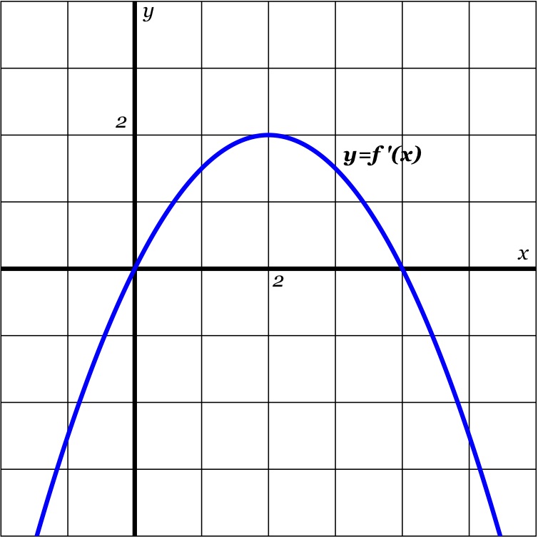
The graph of \(y = f'(x)\) is given below in Figure 2.110.
Figure2.110.A graph of \(y = f'(x)\text{.}\)
Your task is to determine as much information as possible about \(f\) (especially near the value \(a = 2\)) by responding to the questions below.
Find a formula for the tangent line approximation, \(L(x)\text{,}\) to \(f\) at the point \((2,-1)\text{.}\)
Use the tangent line approximation to estimate the value of \(f(2.07)\text{.}\) Show your work carefully and clearly.
Sketch a graph of \(y = f''(x)\text{;}\) label it appropriately.
Is the slope of the tangent line to \(y = f(x)\) increasing, decreasing, or neither when \(x = 2\text{?}\) Explain.
Sketch a possible graph of \(y = f(x)\) near \(x = 2\text{.}\) Include a sketch of \(y=L(x)\) (found in part (a)). Explain how you know the graph of \(y = f(x)\) looks like you have drawn it.
Does your estimate in (b) over- or under-estimate the true value of \(f(2.07)\text{?}\) Why?
Hint.
Find the value of \(f'(2)\) from the given graph of \(y=f'(x)\text{.}\)
Remember that \(f(2.07) \approx L(2.07)\text{.}\)
\(f''(x)\) is the derivative of \(f'(x)\text{.}\)
Is \(f'\) increasing, decreasing, or neither when \(x = 2\text{?}\)
Draw \(y = L(x)\) first. Then think about options for \(f\) relative to the graph of \(L\text{.}\)
Does the tangent line at \(x=2\) lie above or below the graph of \(y = f(x)\) at \(x=2.07\text{?}\)
The leftmost image below shows a possible graph of \(y = f(x)\) near \(x = 2\text{,}\) along with the tangent line \(y = L(x)\) through \((2, f(2))\text{.}\)
It is an overestimate.
Solution.
Since \(f(2) = -1\) and \(f'(2) = 2\text{,}\) we have \(L(x) = -1 + 2(x-2)\text{.}\)
Using our work in (a), \(f(2.07) \approx L(2.07) = -1 + 2(2.07-2) = -1 + 2\cdot 0.07 = -0.86\text{.}\)
The slope of the tangent line to \(y = f(x)\) is increasing for \(x \lt 2\) because \(y = f'(x)\) is an increasing function on this interval. Similarly, for \(x > 2\text{,}\) the slope of the tangent line to \(y = f(x)\) is decreasing. Right at \(x = 2\text{,}\) the slope of the tangent line to \(y = f(x)\) is neither increasing nor decreasing. This can also be seen in the sketch of \(y=f''(x)\text{,}\) where we have \(f''(x)\) decreasing with a root at \(2\) (so \(f''\) is positive to the left and negative to the right of \(x=2\)).
The leftmost image below shows a possible graph of \(y = f(x)\) near \(x = 2\text{,}\) along with the tangent line \(y = L(x)\) through \((2, f(2))\text{.}\)
Note that \(y = f(x)\) is concave up for \(x \lt 2\) since \(f'\) is increasing on that interval, and \(y = f(x)\) is concave down for \(x > 2\) since \(f'\) is decreasing there. Hence \(y = f(x)\) changes from concave up to concave down right at \(x = 2\text{,}\) which is also the point near 2 where the graph of \(y = f(x)\) is steepest.
We also observe that \(f\) is decreasing for \(x \lt 0\) and \(x\gt4\) since \(f'\) is negative on those intervals. Likewise, \(f\) is increasing for \(0\lt x\lt 4\) because \(f'\) is positive on that interval.
As noted in part (e), the function \(f\) is concave down for \(x>2\text{.}\) Consequently, the tangent line approximation for \(f\) at \(x=2\) lies above the graph of \(y=f(x)\) to the right of this point. In other words, \(L(2.07)\gt f(2.07)\text{,}\) and our estimate in (b) was an overestimate for the true value of \(f(2.07)\text{.}\)
The idea that a differentiable function looks linear and can be well-approximated by a linear function is an important one that is widely applied in calculus. For example, it is possible to develop an effective algorithm to estimate the zeroes of a function by approximating the function with its local linearization. Local linearity also helps us to make further sense of certain challenging limits. For instance, the limit
is indeterminate, because both its numerator and denominator tend to 0. While there is no algebra that we can do to simplify \(\frac{\sin(x)}{x}\text{,}\) it is straightforward to show that the linearization of \(f(x) = \sin(x)\) at the point \((0,0)\) is given by \(L(x) = x\text{.}\) Hence \(\sin(x)\approx x\) for values of \(x\) near 0, and therefore
The tangent line to a differentiable function \(y = f(x)\) at the point \((a,f(a))\) is given in point-slope form by the equation
\begin{equation*}
y - f(a) = f'(a)(x-a)\text{.}
\end{equation*}
The principle of local linearity tells us that if we zoom in on a point where a function \(y = f(x)\) is differentiable, the function will be indistinguishable from its tangent line. That is, a differentiable function looks linear when viewed up close. We rename the tangent line to be the function \(y = L(x)\text{,}\) where \(L(x) = f(a) + f'(a)(x-a)\text{.}\) Thus, \(f(x) \approx L(x)\) for all \(x\) near \(x = a\text{.}\)
If we know the tangent line approximation \(L(x) = f(a) + f'(a)(x-a)\) to a function \(f\text{,}\) then because \(L(a) = f(a)\) and \(L'(a) = f'(a)\text{,}\) we also know the values of both the function and its derivative at the point where \(x = a\text{.}\) In other words, the linear approximation tells us the height and slope of the original function. If in addition we know the value of \(f''(a)\text{,}\) we then know whether the tangent line lies above or below the graph of \(y = f(x)\text{,}\) depending on the concavity of \(f\text{.}\)
Exercises2.9.4Exercises
1.Approximating \(\sqrt{x}\).
Use linear approximation to approximate \(\sqrt {49.2}\) as follows.
Let \(f(x) = \sqrt x\text{.}\) The equation of the tangent line to \(f(x)\) at \(x = 49\) can be written in the form \(y = mx+b\text{.}\) Compute \(m\) and \(b\text{.}\)
\(m=\)
\(b=\)
Using this find the approximation for \(\sqrt {49.2}\text{.}\)
Answer:
2.Local Linearization of a Graph.
The figure below shows \(f(x)\) and its local linearization at \(x=a\text{,}\)\(y = 2 x - 3\text{.}\) (The local linearization is shown in blue.)
What is the value of \(a\text{?}\)
\(a =\)
What is the value of \(f(a)\text{?}\)
\(f(a) =\)
Use the linearization to approximate the value of \(f(4.5)\text{.}\)
\(f(4.5) =\)
Is the approximation an under- or overestimate?
(Enter under or over.)
3.Estimating With the Local Linearization.
Suppose that \(f(x)\) is a function with \(f(145) = 64\) and \(f'(145) = 8\text{.}\) Estimate \(f(145.5)\text{.}\)
\(f(145.5) =\)
4.Predicting Behavior From the Local Linearization.
The temperature, \(H\text{,}\) in degrees Celsius, of a cup of coffee placed on the kitchen counter is given by \(H = f(t)\text{,}\) where \(t\) is in minutes since the coffee was put on the counter.
(a) Is \(f'(t)\) positive or negative?
positive
negative
(Be sure that you are able to give a reason for your answer.)
(b) What are the units of \(f'(35)\text{?}\)
Suppose that \(|f'(35)| = 0.6\) and \(f(35) = 59\text{.}\) Fill in the blanks (including units where needed) and select the appropriate terms to complete the following statement about the temperature of the coffee in this case.
At minutes after the coffee was put on the counter, its
derivative
temperature
change in temperature
is and will
increase
decrease
by about in the next 30 seconds.
5.Using the Local Linearization to Analyze a Function.
A certain function \(y=p(x)\) has its local linearization at \(a = 3\) given by \(L(x) = -2x + 5\text{.}\)
What are the values of \(p(3)\) and \(p'(3)\text{?}\) Why?
Estimate the value of \(p(2.79)\text{.}\)
Suppose that \(p''(3) = 0\) and you know that \(p''(x) \lt 0\) for \(x \lt 3\text{.}\) Is your estimate in (b) too large or too small?
Suppose that \(p''(x) \gt 0\) for \(x \gt 3\text{.}\) Use this fact and the additional information above to sketch an accurate graph of \(y = p(x)\) near \(x = 3\text{.}\) Include a sketch of \(y = L(x)\) in your work.
6.Using the Local Linearization with Physical Context.
A potato is placed in an oven, and the potato’s temperature \(F\) (in degrees Fahrenheit) at various points in time is taken and recorded in the following table. Time \(t\) is measured in minutes.
Table2.111.Temperature data for the potato.
\(t\)
\(F(t)\)
\(0\)
\(70\)
\(15\)
\(180.5\)
\(30\)
\(251\)
\(45\)
\(296\)
\(60\)
\(324.5\)
\(75\)
\(342.8\)
\(90\)
\(354.5\)
Use a central difference to estimate \(F'(60)\text{.}\) Use this estimate as needed in subsequent questions.
Find the local linearization \(y = L(t)\) to the function \(y = F(t)\) at the point where \(a = 60\text{.}\)
Determine an estimate for \(F(63)\) by employing the local linearization.
Do you think your estimate in (c) is too large or too small? Why?
7.Local Linearity and the Position of a Moving Object.
An object moving along a straight line path has a differentiable position function \(y = s(t)\text{;}\)\(s(t)\) measures the object’s position relative to the origin at time \(t\text{.}\) It is known that at time \(t = 9\) seconds, the object’s position is \(s(9) = 4\) feet (i.e., 4 feet to the right of the origin). Furthermore, the object’s instantaneous velocity at \(t = 9\) is \(-1.2\) feet per second, and its acceleration at the same instant is \(0.08\) feet per second per second.
Use local linearity to estimate the position of the object at \(t = 9.34\text{.}\)
Is your estimate likely too large or too small? Why?
In everyday language, describe the behavior of the moving object at \(t = 9\text{.}\) Is it moving toward the origin or away from it? Is its velocity increasing or decreasing?
8.Estimating a Function Through its Derivative.
For a certain function \(f\text{,}\) its derivative is known to be \(f'(x) = (x-1)e^{-x^2}\text{.}\) Note that you do not know a formula for \(y = f(x)\text{.}\)
At what \(x\)-value(s) is \(f'(x) = 0\text{?}\) Justify your answer algebraically, but include a graph of \(f'\) to support your conclusion.
Reasoning graphically, for what intervals of \(x\)-values is \(f''(x) \gt 0\text{?}\) What does this tell you about the behavior of the original function \(f\text{?}\) Explain.
Assuming that \(f(2) = -3\text{,}\) estimate the value of \(f(1.88)\) by finding and using the tangent line approximation to \(f\) at \(x=2\text{.}\) Is your estimate larger or smaller than the true value of \(f(1.88)\text{?}\) Justify your answer.