CC The Second Derivative

🔗

Section 1.7 The Second Derivative

🔗

Motivating Questions

How does the derivative of a function tell us whether the function is increasing or decreasing at a point or on an interval?
What can we learn by taking the derivative of the derivative (the second derivative) of a function $f ?$
What does it mean to say that a function is concave up or concave down? How are these characteristics connected to certain properties of the derivative of the function?
What are the units of the second derivative? How do they help us understand the rate of change of the rate of change?

🔗

Supplemental Videos.

🔗

The main topics of this section are also presented in the following videos:

The Second Derivative
³¹
unl.yuja.com/V/Video?v=7114223&node=34303244&a=24060156&autoplay=1
Concavity
³²
unl.yuja.com/V/Video?v=7114224&node=34303291&a=165064445&autoplay=1
Acceleration
³³
unl.yuja.com/V/Video?v=7114225&node=34303221&a=169906632&autoplay=1

🔗

Given a differentiable function

y = f (x),

we know that its derivative,

y = f^{'} (x),

is a related function whose output at

x = a

tells us the slope of the tangent line to

y = f (x)

at the point

(a, f (a)) .

That is,

y

-coordinates on the derivative graph tell us the values of slopes on the original function’s graph.

🔗

At a point where

f^{'} (x)

is positive, the slope of the tangent line to

f

is positive. Therefore, on an interval where

f^{'} (x)

is positive, the function

f

is increasing (or rising). Similarly, if

f^{'} (x)

is negative on an interval, the graph of

f

is decreasing (or falling).

🔗

The derivative of

f

tells us not only whether the function

f

is increasing or decreasing on an interval, but also how the function

f

is increasing or decreasing. Look at the two tangent lines shown below in Figure 1.75. We see that at point

A

the value of

f^{'} (x)

is positive and relatively close to zero, and at that point the graph is rising slowly. By contrast, at point

B,

the derivative is negative and relatively large in absolute value, and

f

is decreasing rapidly at

B .

🔗
Figure 1.75. Two tangent lines on a graph.

🔗

Besides asking whether the value of the derivative function is positive or negative and whether it is large or small, we can also ask “how is the derivative changing?”

🔗

Because the derivative,

y = f^{'} (x),

is itself a function, we can consider taking its derivative — the derivative of the derivative — and ask “what does the derivative of the derivative tell us about how the original function behaves?” We start with an investigation of a moving object.

Example 1.76.

The position of a car driving along a straight road at time

t

in minutes is given by the function

y = s (t)

that is pictured below in Figure 1.77. The car’s position function has units measured in thousands of feet. For instance, the point

(2, 4)

on the graph indicates that after 2 minutes, the car has traveled 4000 feet.

Figure 1.77. The graph of $y = s (t),$ the position of the car (measured in thousands of feet from its starting location) at time $t$ in minutes.

In everyday language, describe the behavior of the car over the provided time interval. In particular, you should carefully discuss what is happening on each of the time intervals $[0, 1],$ $[1, 2],$ $[2, 3],$ $[3, 4],$ and $[4, 5],$ plus provide commentary overall on what the car is doing on the interval $[0, 12] .$
Sketch a careful, accurate graph of $y = s^{'} (t) .$
What is the meaning of the function $y = s^{'} (t)$ in the context of the given problem? What can we say about the car’s behavior when $s^{'} (t)$ is positive? when $s^{'} (t)$ is zero? when $s^{'} (t)$ is negative?
Rename the function you graphed in (b) to be called $y = v (t) .$ Describe the behavior of $v$ in words, using phrases like “ $v$ is increasing on the interval $\dots$ ” and “ $v$ is constant on the interval $\dots .$ ”
Sketch a graph of the function $y = v^{'} (t) .$ Write at least one sentence to explain how the behavior of $v^{'} (t)$ is connected to the graph of $y = v (t) .$

Hint.

Can you estimate the car’s speed at different times? Does it ever stop or change direction? How can you tell?
What are the units on $s^{'} ?$ When is the slope of the tangent line to $s$ positive, zero, or negative? How big does it get?
What are the units on $s^{'} ?$ When is the value of the derivative positive, zero, or negative, and how does that relate to the direction the car is traveling at that time?
When does your graph in (b) have positive slope? Negative slope? Zero slope?
Look at your graph of $y = v (t)$ from (b). What do the slopes of the tangent lines to $v$ tell you about the values of $v^{'} (t) ?$

Answer.

The car starts out not moving and then speeds up for a minute as it travels about $1300$ feet forward before starting to slow down in the second minute, coming to a stop at time $t = 2$ minutes at a point $4000$ feet from its starting position. The car is stopped during the third minute. This three-minute pattern repeats for the full $12$ minutes, at which point the car is $16, 000$ feet from its starting position, having always traveled in the same direction along the road.
Figure 1.78. The graph of $y = s^{'} (t),$ showing the velocity of the car, in thousands of feet per minute, after $t$ minutes.
$s^{'}$ describes the velocity of the car, in $1000$ ft/min, after $t$ minutes of driving. The car moves forward when $s^{'} (t)$ is positive, moves backward when $s^{'} (t)$ is negative, and is stopped when $s^{'} (t) = 0 .$
$v$ is increasing on the intervals $(0, 1.1),$ $(3, 4.1),$ $(6, 7.1),$ and $(9, 10.1) .$ $v$ is decreasing on the intervals $(1.1, 2),$ $(4.1, 5),$ $(7.1, 8),$ and $(10.1, 11) .$ $v$ is constant on the intervals $(2, 3),$ $(5, 6),$ $(8, 9),$ and $(11, 12) .$
Figure 1.79. The graph of $y = v^{'} (t),$ showing the acceleration of the car, in thousands of feet per minute per minute, after $t$ minutes.
As seen in the graph above: $v^{'}$ is positive whenever $v$ is increasing; $v^{'}$ is negative whenever $v$ is decreasing; $v^{'}$ is zero whenever $v$ is constant.

Solution.

At time $t = 0,$ the car is at rest but gradually accelerates to a speed of about $6000$ ft/min as it drives about $1300$ feet during the first minute of travel. The car reaches its peak speed of about $7000$ ft/min just after the time $t = 1$ minute (and again just after the points $t = 4,$ $t = 7,$ and $t = 10$ minutes). In the second minute, the car gradually slows back down, coming to a stop about $4000$ feet from where it started. It waits there for a minute (between $t = 2$ minutes and $t = 3$ minutes) before continuing to drive in the same direction as before. At this point, the car again gradually accelerates to a speed of about $6000$ ft/min by the end of the fourth minute, at which point it has driven around $5300$ feet since starting out. During the fifth minute, the car gradually slows back to a stop after traveling an additional $2700$ feet. This pattern of starts and stops continues for a total of $12$ minutes, by which time the car has traveled a total of $16, 000$ feet from its starting point.
Figure 1.80. The graph of $y = s^{'} (t),$ showing the velocity of the car, in thousands of feet per minute, after $t$ minutes.
The car is stopped at $t = 0$ and $t = 12$ minutes, as well as on the intervals $(2, 3),$ $(5, 6),$ $(8, 9),$ and $(11, 12) .$ The value of $s^{'}$ at these times is $0$ ft/min. In the minute or so after each of the points $t = 0,$ $t = 3,$ $t = 6,$ and $t = 9,$ the car gradually accelerates to a speed of about $7000$ ft/min, and then gradually slows back down, reaching a speed of $0$ ft/min by the times $t = 2,$ $t = 5,$ $t = 8,$ and $t = 11$ minutes. While the car is speeding up, the graph of $y = s^{'} (t)$ has a positive slope; while the car is slowing down, the graph of $y = s^{'} (t)$ has a negative slope. When the car is traveling at a constant speed (of $0$ ft/min), the graph of $y = s^{'} (t)$ is horizontal.
The derivative function $s^{'}$ describes the velocity of the car, in thousands of feet per minute, after $t$ minutes of driving. The car moves forward when $s^{'} (t)$ is positive, moves backward when $s^{'} (t)$ is negative, and is stopped when $s^{'} (t) = 0 .$
$v$ is increasing from $0$ ft/min to $7000$ ft/min approximately on the $66$ -second intervals $(0, 1.1),$ $(3, 4.1),$ $(6, 7.1),$ and $(9, 10.1) .$ $v$ is decreasing from $7000$ ft/min to $0$ ft/min approximately on the $54$ -second intervals $(1.1, 2),$ $(4.1, 5),$ $(7.1, 8),$ and $(10.1, 11) .$ $v$ is constant at $0$ ft/min on the $1$ -minute intervals $(2, 3),$ $(5, 6),$ $(8, 9),$ and $(11, 12) .$
Figure 1.81. The graph of $y = v^{'} (t),$ showing the acceleration of the car, in thousands of feet per minute per minute, after $t$ minutes.
As seen in the graph above: $v^{'}$ is positive whenever $v$ is increasing; $v^{'}$ is negative whenever $v$ is decreasing; $v^{'}$ is zero whenever $v$ is constant. Since the units of $v^{'}$ are thousands of feet per minute squared, we conjecture that the function $v^{'}$ models the acceleration of the car after $t$ minutes of driving. Thus we have positive acceleration whenever the car is speeding up (increasing velocity), negative acceleration whenever the car is slowing down (decreasing velocity), and zero acceleration whenever the car travels at a constant speed (constant velocity).

🔗

Subsection 1.7.1 Increasing, Decreasing, or Neither

🔗

So far, we have used the words increasing and decreasing intuitively to describe a function’s graph. Here we define these terms more formally.

🔗

Increasing and Decreasing Functions.

🔗

Given a function

f (x)

defined on the interval

(a, b),

we say that

f

is increasing on

(a, b)

provided that

f (x) < f (y)

whenever

a < x < y < b .

Similarly, we say that

f

is decreasing on

(a, b)

provided that

f (x) > f (y)

whenever

a < x < y < b .

🔗

Simply put, an increasing function is one that is rising as we move from left to right along the graph, and a decreasing function is one that falls as the value of the input increases. If the function has a derivative, the sign of the derivative tells us whether the function is increasing or decreasing.

🔗

Let

f

be a function that is differentiable on an interval

(a, b) .

If the function

f

is increasing on

(a, b)

then

f^{'} (x) \geq 0

for every

x

in the interval

(a, b) .

Conversely, if

f^{'} (x) > 0

for every

x

in the interval, then the function

f

must be increasing on the interval. Notice that we have to have the derivative strictly positive to conclude that the function is increasing. Letting

f

be a constant function shows that if the derivative can be zero, then the function need not be increasing. Also, knowing the function is increasing is not enough to conclude that the derivative is positive. The function

f (x) = x^{3}

is increasing on

(- 1, 1)

but

f^{'} (0) = 0 .

🔗

Similarly, if the function

f

is decreasing on

(a, b)

then

f^{'} (x) \leq 0

for every

x

in the interval

(a, b) .

Conversely, if

f^{'} (x) < 0

for every

x

in the interval, then the function

f

must be decreasing on the interval.

🔗

For example, the function pictured below in Figure 1.82 is increasing on the entire interval

- 2 < x < 0 .

Note that at both

x = \pm 2

and

x = 0,

we say that

f

is neither increasing nor decreasing, because

f^{'} (x) = 0

at these values.

🔗
Figure 1.82. A function that is decreasing on the intervals $- 3 < x < - 2$ and $0 < x < 2$ and increasing on $- 2 < x < 0$ and $2 < x < 3 .$

🔗

Subsection 1.7.2 The Second Derivative

🔗

We are now accustomed to investigating the behavior of a function by examining its derivative. The derivative of a function

f

is a new function given by the rule

f^{'} (x) = lim_{h \to 0} \frac{f (x + h) - f (x)}{h} .

🔗

Because

f^{'}

is itself a function, it is perfectly feasible for us to consider the derivative of the derivative, which is the new function

y = [f^{'} (x)]^{'} .

We call this resulting function the second derivative of $f,$ and denote the second derivative by

y = f^{″} (x) .

Consequently, we will sometimes call

f^{'}

“the first derivative” of

f,

rather than simply “the derivative” of

f .

🔗

Second Derivative.

🔗

The second derivative is defined by applying the limit definition of the derivative to the first derivative. That is,

f^{″} (x) = lim_{h \to 0} \frac{f^{'} (x + h) - f^{'} (x)}{h} .

🔗

We read “

f^{″} (x)

” as “

f

-double prime of

x

”, or as “the second derivative of

f

”.

🔗

The meaning of the derivative function still holds, so when we compute

f^{″} (x),

this new function measures slopes of tangent lines to the curve

y = f^{'} (x),

as well as the instantaneous rate of change of

y = f^{'} (x) .

In other words, just as the first derivative measures the rate at which the original function changes, the second derivative measures the rate at which the first derivative changes. The second derivative will help us understand how the rate of change of the original function is itself changing.

🔗

Subsection 1.7.3 Concavity

🔗

In addition to asking whether a function is increasing or decreasing, it is also natural to inquire how a function is increasing or decreasing. There are three basic behaviors that an increasing function can demonstrate on an interval, as pictured below in Figure 1.83: the function can increase more and more rapidly, it can increase at the same rate, or it can increase in a way that is slowing down. Fundamentally, we are beginning to think about how a particular curve bends, with the natural comparison being made to lines, which don’t bend at all. More than this, we want to understand how the bend in a function’s graph is tied to behavior characterized by the first derivative of the function.

🔗
Figure 1.83. Three functions that are all increasing, but doing so at an increasing rate, at a constant rate, and at a decreasing rate, respectively.

🔗

On the leftmost curve in Figure 1.83, draw a sequence of tangent lines to the curve. As we move from left to right, the slopes of those tangent lines will increase. Therefore, the rate of change of the pictured function is increasing, and this explains why we say this function is increasing at an increasing rate. For the rightmost graph in Figure 1.83, observe that as

x

increases, the function increases, but the slopes of the tangent lines decrease. This function is increasing at a decreasing rate.

🔗

Similar options hold for how a function can decrease. Here we must be extra careful with our language, because decreasing functions involve negative slopes.

³⁴

Negative numbers present an interesting tension between common language and mathematical language. For example, it can be tempting to say that “

- 100

is bigger than

- 2 .

” But we must remember that “greater than” describes how numbers lie on a number line:

x > y

provided that

x

lies to the right of

y .

So of course,

- 100

is less than

- 2 .

Informally, it might be helpful to say that “

- 100

is more negative than

- 2 .

”

When a function’s values are negative, and those values get more negative as the input increases, the function must be decreasing.

🔗
Figure 1.84. From left to right, three functions that are all decreasing, but doing so in different ways.

🔗

Now consider the three graphs shown above in Figure 1.84. The middle graph clearly depicts a function decreasing at a constant rate. Now draw a sequence of tangent lines on the first curve. We see that the slopes of these lines get closer to zero — meaning they get less and less negative — as we move from left to right. That means that the values of the first derivative, while all negative, are increasing, and thus we say that the leftmost curve is decreasing at an increasing rate.

🔗

This leaves only the rightmost curve in Figure 1.84 to consider. For that function, the slopes of the tangent lines are negative throughout the pictured interval, but as we move from left to right, the slopes get more and more negative as they get steeper. Hence the slope of the curve is decreasing, and we say that the function is decreasing at a decreasing rate.

🔗

We now introduce the notion of concavity, which provides simpler language to describe these behaviors. When a curve opens upward on a given interval, like the parabola

y = x^{2}

or the exponential growth function

y = e^{x},

we say that the curve is concave up on that interval. Likewise, when a curve opens down, like the parabola

y = - x^{2}

or the negative exponential function

y = - e^{x},

we say that the function is concave down. Concavity is linked to both the first and second derivatives of the function.

🔗

In Figure 1.85 below, we see two functions and a sequence of tangent lines to each. The lefthand plot shows a function that is concave up; observe that here the tangent lines always lie below the curve itself, and the slopes of the tangent lines are increasing as we move from left to right. In other words, the graph of

y = f (x)

is concave up on the interval shown because its derivative,

f^{'},

is increasing on that interval. Similarly, the righthand plot in Figure 1.85 depicts a function that is concave down; in this case, we see that the tangent lines alway lie above the curve and that the slopes of the tangent lines are decreasing as we move from left to right. The fact that its derivative,

f^{'},

is decreasing makes

f

concave down on the interval shown.

🔗
Figure 1.85. At left, a function that is concave up; at right, one that is concave down.

🔗

We state these most recent observations formally as the definitions of the terms concave up and concave down.

🔗

Concavity.

🔗

Let

f

be a differentiable function on an interval

(a, b) .

Then

f

is concave up on

(a, b)

if and only if

f^{'}

is increasing on

(a, b);

f

is concave down on

(a, b)

if and only if

f^{'}

is decreasing on

(a, b) .

Example 1.86.

The position of a car driving along a straight road at time

t

in minutes is given by the function

y = s (t)

that is pictured below in Figure 1.87. The car’s position function has units measured in thousands of feet. Remember that you worked with this function and sketched graphs of

y = v (t) = s^{'} (t)

and

y = v^{'} (t) = s^{″} (t)

earlier, in Example 1.76.

Figure 1.87. The graph of $y = s (t),$ the position of the car (measured in thousands of feet from its starting location) at time $t$ in minutes.

On what intervals is the position function $y = s (t)$ increasing? Decreasing? Why?
On which intervals is the velocity function $y = v (t) = s^{'} (t)$ increasing? Decreasing? Neither? Why?
Acceleration is defined to be the instantaneous rate of change of velocity, as the acceleration of an object measures the rate at which the velocity of the object is changing. Say that the car’s acceleration function is named $a (t) .$ How is $a (t)$ computed from $v (t) ?$ How is $a (t)$ computed from $s (t) ?$ Explain.
What can you say about $s^{″}$ whenever $s^{'}$ is increasing? Why?
Using only the words increasing, decreasing, constant, concave up, concave down, and linear, complete the following sentences. For the position function $s$ with velocity $v$ and acceleration $a,$
- on an interval where $v$ is positive, $s$ is .
- on an interval where $v$ is negative, $s$ is .
- on an interval where $v$ is zero, $s$ is .
- on an interval where $a$ is positive, $v$ is .
- on an interval where $a$ is negative, $v$ is .
- on an interval where $a$ is zero, $v$ is .
- on an interval where $a$ is positive, $s$ is .
- on an interval where $a$ is negative, $s$ is .
- on an interval where $a$ is zero, $s$ is .

Hint.

Remember that a function is increasing on an interval if and only if its first derivative is positive on the interval.
See (a).
Remember that the first derivative of a function measures its instantaneous rate of change.
Think about how $s^{″} (t) = [s^{'} (t)]^{'} .$
Be very careful with your letters: $s,$ $v,$ and $a .$

Answer.

Increasing: $0 < t < 2,$ $3 < t < 5,$ $6 < t < 8,$ and $9 < t < 11 .$ Decreasing: never.
Velocity is increasing on $0 < t < 1.1,$ $3 < t < 4.1,$ $6 < t < 7.1,$ and $9 < t < 10.1;$ $y = v (t)$ is decreasing on $1.1 < t < 2,$ $4.1 < t < 5,$ $7.1 < t < 8,$ and $10.1 < t < 11 .$ Velocity is neither increasing nor decreasing (i.e. the velocity is constant) on $2 < t < 3,$ $5 < t < 6,$ $8 < t < 9,$ and $11 < t < 12 .$
$a (t) = v^{'} (t)$ and $a (t) = s^{″} (t) .$
$s^{″} (t)$ is positive since $s^{'} (t)$ is increasing.
- increasing.
- decreasing.
- constant.
- increasing.
- decreasing.
- constant.
- concave up.
- concave down.
- linear.

Solution.

The position function $y = s (t)$ is increasing on the intervals $0 < t < 2,$ $3 < t < 5,$ $6 < t < 8,$ and $9 < t < 11$ because $s^{'} (t)$ is positive at every point in such intervals. Furthermore, $s (t)$ is never decreasing because its derivative is never negative.
The velocity function $y = v (t)$ appears to be increasing on the intervals $0 < t < 1.1,$ $3 < t < 4.1,$ $6 < t < 7.1,$ and $9 < t < 10.1 .$ This is because the curve $y = s (t)$ is concave up on these intervals, which corresponds to an increasing first derivative $y = s^{'} (t) .$ Similarly, $y = v (t)$ appears to be decreasing on the intervals $1.1 < t < 2,$ $4.1 < t < 5,$ $7.1 < t < 8,$ and $10.1 < t < 11 .$ This is due to the curve $y = s (t)$ being concave down on these intervals, corresponding to a decreasing first derivative $y = s^{'} (t) .$ On the intervals $2 < t < 3,$ $5 < t < 6,$ $8 < t < 9,$ and $11 < t < 12,$ the curve $y = s (t)$ is constant, and thus linear, so $s$ is neither concave up nor concave down. On these intervals, then, the velocity function is constant.
Since $a (t)$ is the instantaneous rate of change of $v (t),$ we can say $a (t) = v^{'} (t) .$ Moreover, because $v (t) = s^{'} (t),$ it follows that $a (t) = v^{'} (t) = [s^{'} (t)]^{'} = s^{″} (t),$ so acceleration is the second derivative of position.
Since $s^{″} (t)$ is the first derivative of $s^{'} (t),$ then whenever $s^{'} (t)$ is increasing, $s^{″} (t)$ must be positive.
For the position function $s (t)$ with velocity $v (t)$ and acceleration $a (t),$
- on an interval where $v (t)$ is positive, $s (t)$ is increasing.
- on an interval where $v (t)$ is negative, $s (t)$ is decreasing.
- on an interval where $v (t)$ is zero, $s (t)$ is constant.
- on an interval where $a (t)$ is positive, $v (t)$ is increasing.
- on an interval where $a (t)$ is negative, $v (t)$ is decreasing.
- on an interval where $a (t)$ is zero, $v (t)$ is constant.
- on an interval where $a (t)$ is positive, $s (t)$ is concave up.
- on an interval where $a (t)$ is negative, $s (t)$ is concave down.
- on an interval where $a (t)$ is zero, $s (t)$ is linear.

🔗

Exploring the context of position, velocity, and acceleration is an excellent way to understand how a function, its first derivative, and its second derivative are related to one another. In Example 1.86 that we just finished, we can replace

s,

v,

and

a

with an arbitrary function

f

and its derivatives

f^{'}

and

f^{″},

and essentially all the same observations hold. In particular, note that the following are equivalent: on an interval where the graph of

y = f (x)

is concave up,

f^{'}

is increasing and

f^{″}

is positive. Likewise, on an interval where the graph of

y = f (x)

is concave down,

f^{'}

is decreasing and

f^{″}

is negative.

Example 1.88.

A potato is placed in an oven, and the potato’s temperature

F

(in degrees Fahrenheit) at various points in time is taken and recorded below in Table 1.89. Time

t

is measured in minutes. We also provide data for

F^{'} (t)

in Table 1.90 below on the right.

$t$	$F (t)$
$0$	$70$
$15$	$180.5$
$30$	$251$
$45$	$296$
$60$	$324.5$
$75$	$342.8$
$90$	$354.5$

Table 1.89. Select values of

F (t) .

$t$	$F^{'} (t)$
$0$	NA
$15$	$6.03$
$30$	$3.85$
$45$	$2.45$
$60$	$1.56$
$75$	$1.00$
$90$	NA

Table 1.90. Select values of

F^{'} (t) .

What are the units on the values of $F^{'} (t) ?$
Use the formula

$g^{'} (a) \approx \frac{g (a + h) - g (a - h)}{2 h}$

(commonly called a central difference) to estimate the value of $F^{″} (30) .$
In terms of the potato’s temperature, what is the meaning of the value of $F^{″} (30)$ that you have computed in (b)? Write several careful sentences that discuss (with appropriate units) the values of $F (30),$ $F^{'} (30),$ and $F^{″} (30),$ and explain the overall behavior of the potato’s temperature at this point in time.
Overall, is the potato’s temperature increasing at an increasing rate, increasing at a constant rate, or increasing at a decreasing rate? Why?

Hint.

Remember that the derivative’s units are “units of output per unit of input.”
Try using $g = F^{'}$ and $a = 30 .$ Choose a value for $h$ that works with the data available in Table 1.90. Note that a central difference just calculates the slope of a secant line between two input values whose midpoint is $a .$
For each of the values $F^{'} (30)$ and $F^{″} (30),$ think about what they tell you about expected upcoming behavior in $F (t)$ and $F^{'} (t),$ respectively.
Think about concavity.

Answer.

Degrees Fahrenheit per minute.
$F^{″} (30) \approx - 0.119 .$
At the moment $t = 30,$ the temperature of the potato is $251$ degrees; its temperature is rising at a rate of $3.85$ degrees per minute; and the rate at which the temperature is rising is falling at a rate of $0.119$ degrees per minute per minute.
Increasing at a decreasing rate.

Solution.

$F^{'} (t)$ has units measured in degrees Fahrenheit per minute.
Using a central difference,

$F^{″} (30) \approx \frac{F^{'} (45) - F^{'} (15)}{30} = \frac{2.45 - 6.03}{30} \approx - 0.119 .$
The values $F (30) = 251,$ $F^{'} (30) = 3.85,$ and $F^{″} (30) \approx - 0.119$ (which is measured in degrees per minute per minute), tell us that at the moment $t = 30$ minutes: the temperature of the potato is $251$ degrees, its temperature is rising at a rate of $3.85$ degrees per minute, and the rate at which the temperature is rising is falling at a rate of $0.119$ degrees per minute per minute. That is, even though the temperature is still rising, it is doing so at a slower and slower rate. At $t = 31,$ we expect that the rate of increase of the potato’s temperature would have dropped to about $3.73$ degrees per minute.
The potato’s temperature is increasing at a decreasing rate because the values of the first derivative of $F$ are positive and decreasing. Equivalently, the value of $F^{″} (t)$ is negative throughout the given time interval.

Example 1.91.

This example builds on our experience and understanding of how to sketch the graph of

y = f^{'} (x)

given the graph of

y = f (x) .

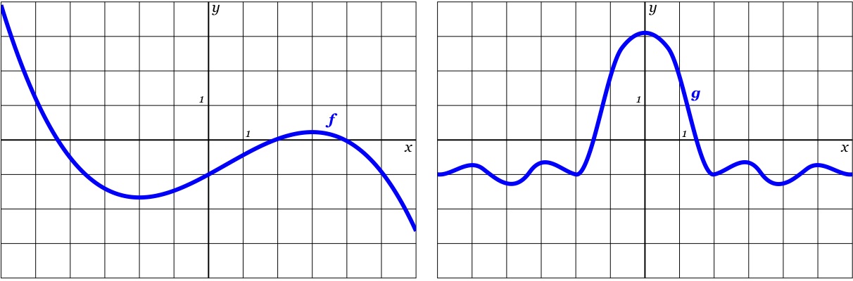
For each of the two functions graphed below in Figure 1.92, sketch the corresponding graphs of the first and second derivatives. In addition, for each, write several careful sentences in the spirit of those in Example 1.86 that connect the behaviors of

f,

f^{'},

and

f^{″}

(or of

g,

g^{'},

and

g^{″}

in the case of the second function). For instance, write something such as

“ $f^{'}$ is on the interval , which is connected to the fact that $f$ is on the same interval , and $f^{″}$ is on the interval.”

but with the blanks filled in. The scale of the grids on the given graphs is

1 \times 1;

be sure to label the scale on each of the graphs you draw, even if it does not change from the original.

Figure 1.92. The graphs of $y = f (x)$ and $y = g (x),$ for two given functions $f$ and $g .$

Hint.

Remember that to plot

y = f^{'} (x),

it is helpful to first identify where

f^{'} (x) = 0 .

Answer.

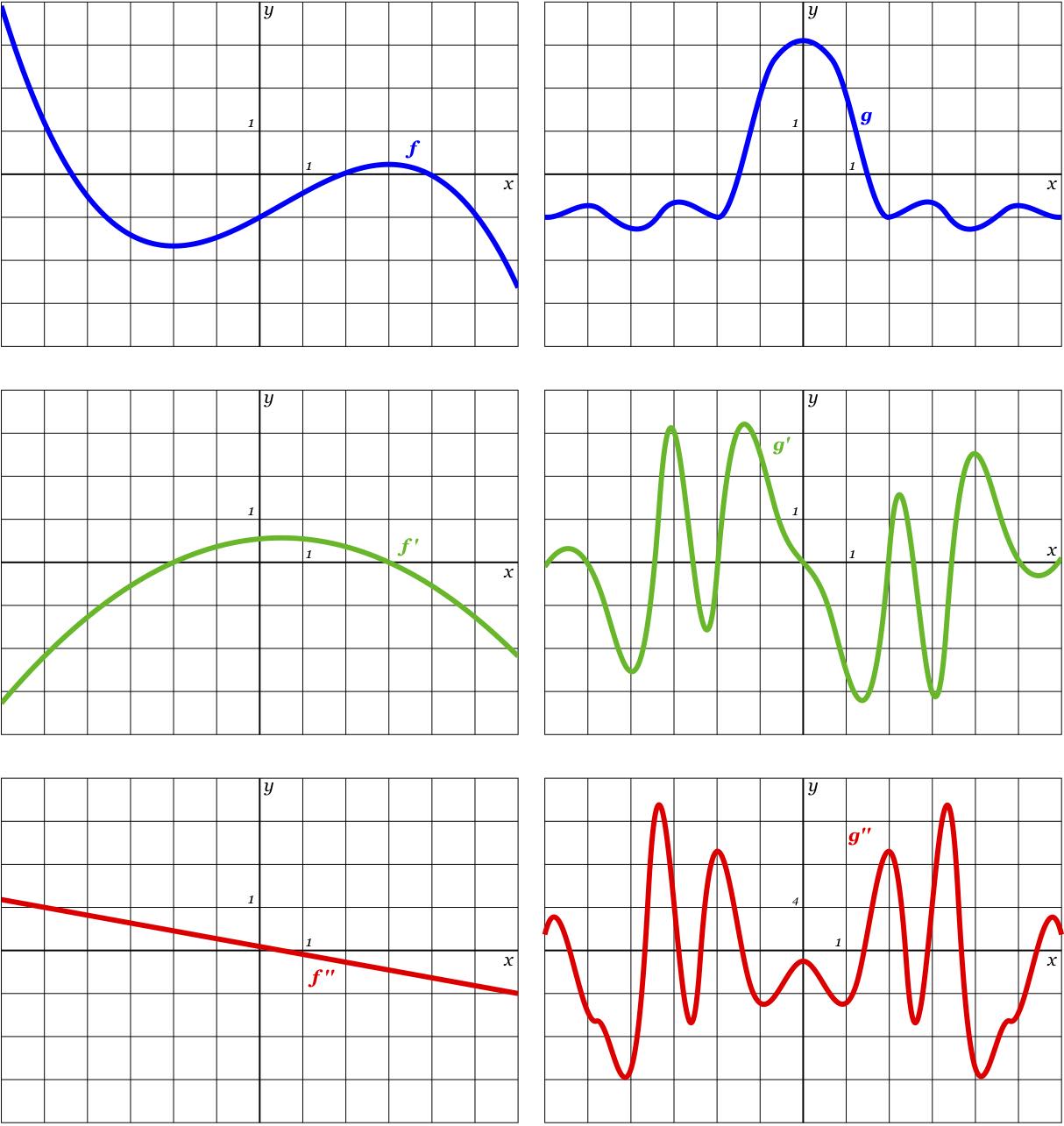
Notice the vertical scale on the graph of

y = g^{″} (x)

has changed, with each grid square now having height

4 .

Solution.

The graphs of

y = f^{'} (x)

and

y = f^{″} (x)

are plotted below the graph of

y = f (x)

on the left. The graphs of

y = g^{'} (x)

and

y = g^{″} (x)

are plotted below the graph of

y = g (x)

on the right. Notice the vertical scale on the graph of

y = g^{″} (x)

has changed, with each grid square now having height

4 .

The graph of $y = f (x)$ is decreasing and concave up on the interval $(- 6, - 2),$ which is connected to the fact that $f^{″}$ is positive, and that $f^{'}$ is negative and increasing on the same interval.
The graph of $y = f (x)$ is increasing and concave up on the interval $(- 2, 0.5),$ which is connected to the fact that $f^{″}$ is positive, and that $f^{'}$ is positive and increasing on the same interval.
The graph of $y = f (x)$ is increasing and concave down on the interval $(0.5, 3),$ which is connected to the fact that $f^{″}$ is negative, and that $f^{'}$ is positive and decreasing on the same interval.
The graph of $y = f (x)$ is decreasing and concave down on the interval $(3, 6),$ which is connected to the fact that $f^{″}$ is negative, and that $f^{'}$ is negative and decreasing on the same interval.
The graph of $y = g (x)$ is increasing and concave up on the (approximate) intervals $(- 6, - 5.5),$ $(- 3.5, - 3),$ $(- 2, - 1.5),$ $(2, 2.2),$ and $(3.5, 4) .$ This is connected to the fact that $g^{″}$ is positive, and that $g^{'}$ is positive and increasing on the same intervals.
The graph of $y = g (x)$ is increasing and concave down on the (approximate) intervals $(- 5.5, - 5),$ $(- 3, - 2.5),$ $(- 1.5, 0),$ $(2.2, 2.5),$ and $(4, 5) .$ This is connected to the fact that $g^{″}$ is negative, and that $g^{'}$ is positive and decreasing on the same intervals.
The graph of $y = g (x)$ is decreasing and concave down on the (approximate) intervals $(- 5, - 4),$ $(- 2.5, - 2.2),$ $(0, 1.5),$ $(2.5, 3),$ and $(5, 5.5) .$ This is connected to the fact that $g^{″}$ is negative, and that $g^{'}$ is negative and decreasing on the same intervals.
The graph of $y = g (x)$ is decreasing and concave up on the (approximate) intervals $(- 4, - 3.5),$ $(- 2.2, - 2),$ $(1.5, 2),$ $(3, 3.5),$ and $(5.5, 6) .$ This is connected to the fact that $g^{″}$ is positive, and that $g^{'}$ is negative and increasing on the same intervals.

🔗

Subsection 1.7.4 Acceleration

🔗

Recall that if the function

s (t)

gave the position of an object at time

t

then

s^{'} (t)

gave the change in position, otherwise known as velocity. That is,

s^{'} (t) = v (t),

where

v (t)

is the velocity function. Using the alternate notation introduced in Section 1.6 we have

\frac{d s}{d t} = v (t) .

🔗

Following this same idea,

v^{'} (t)

gives the change in velocity, more commonly called acceleration. Using derivative notation,

v^{'} (t) = a (t) .

Therefore,

s^{″} (t) = a (t) .

That is, the second derivative of the position function gives acceleration. Using the alternative notation from the previous section 1.6.1, we write

\frac{d^{2} s}{d t^{2}} = a (t) .

³⁵

Notice that in higher order derivatives the exponent occurs in what appear to be different locations in the numerator and denominator. In reality, what is happening is we have

\frac{d^{n}}{d t^{n}}

acting as an operator that takes the

n

th order derivative of the function.

Example 1.93.

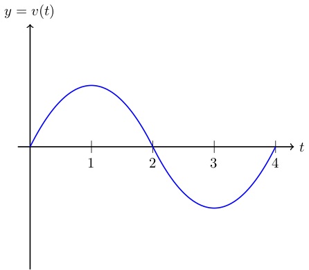
Suppose that an object’s velocity is given by the graph in the figure below.

On what intervals is the acceleration positive?
On what intervals is the object’s position increasing?
Where is the function $s (t)$ concave up?

Figure 1.94. A graph of the velocity of some object.

Hint.

Recall that acceleration is given by the derivative of the velocity function.
Recall that a function is increasing when its derivative is positive. What is the derivative of a position function?
Recall that a function is concave up when its second derivative is positive.

Answer.

$(0, 1) \cup (3, 4) .$
$(0, 2) .$
$(0, 1) \cup (3, 4) .$

Solution.

Recall that acceleration is given by the derivative of the velocity function. Therefore, we can say that acceleration is positive whenever the velocity function is increasing. Since the graph in Figure 1.94 depicts the velocity function, it follows that the object’s acceleration is positive exactly on the intervals $(0, 1)$ and $(3, 4) .$
We know that a function is increasing whenever its derivative is positive, and that velocity, $v,$ is the derivative of position, $s,$ with respect to time, $t .$ Inspection of Figure 1.94 shows that the $v (t)$ is positive only on $(0, 2),$ so the object’s position is increasing on that same interval.
Recall that a function is concave up when its second derivative is positive, which is when its first derivative is increasing. In (a) we saw that the acceleration is positive on $(0, 1) \cup (3, 4);$ as acceleration is the second derivative of position, these are the intervals where the graph of $y = s (t)$ is concave up.

🔗

Subsection 1.7.5 Summary

🔗

A differentiable function $f$ is increasing at a point or on an interval whenever its first derivative is positive, and decreasing whenever its first derivative is negative.
By taking the derivative of the derivative of a function $f,$ we arrive at the second derivative, $f^{″} .$ The second derivative measures the instantaneous rate of change of the first derivative. The sign of the second derivative tells us whether the slope of the tangent line to $f$ is increasing or decreasing.
A differentiable function is concave up whenever its first derivative is increasing (equivalently, whenever its second derivative is positive), and concave down whenever its first derivative is decreasing (equivalently, whenever its second derivative is negative). Examples of functions that are everywhere concave up are $y = x^{2}$ and $y = e^{x};$ examples of functions that are everywhere concave down are $y = - x^{2}$ and $y = - e^{x} .$
The units on the second derivative are “units of output per unit of input per unit of input.” They tell us how the value of the derivative function is changing in response to changes in the input. In other words, the second derivative tells us the rate of change of the rate of change of the original function.

🔗

Exercises 1.7.6 Exercises

🔗

1. Comparing $f, f^{'}, f^{″}$ values.

🔗

Consider the function

f (x)

graphed below.

🔗

For this function, are the following nonzero quantities positive or negative?

🔗

f (3)

positive
negative

🔗

f^{'} (3)

positive
negative

🔗

f^{″} (3)

positive
negative

🔗

(Because this is a multiple choice problem, it will not show which parts of the problem are correct or incorrect when you submit it.)

🔗

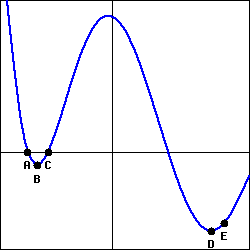
2. Signs of $f, f^{'}, f^{″}$ values.

🔗

At exactly two of the labeled points in the figure below, which shows a function

f,

the derivative

f^{'}

is zero; the second derivative

f^{″}

is not zero at any of the labeled points. Select the correct signs for each of

f,

f^{'}

and

f^{″}

at each marked point.

Point	A	B	C	D	E
$f$	positive zero negative	positive zero negative	positive zero negative	positive zero negative	positive zero negative
$f^{'}$	positive zero negative	positive zero negative	positive zero negative	positive zero negative	positive zero negative
$f^{″}$	positive zero negative	positive zero negative	positive zero negative	positive zero negative	positive zero negative

🔗

3. Acceleration from velocity.

🔗

Suppose that an accelerating car goes from 0 mph to 60.0 mph in five seconds. Its velocity is given in the following table, converted from miles per hour to feet per second, so that all time measurements are in seconds. (Note: 1 mph is 22/15 ft/sec.) Find the average acceleration of the car over each of the first two seconds.

$t$ (s)	0	1	2	3	4	5
$v (t)$ (ft/s)	0.00	30.00	52.00	68.00	80.00	88.00

🔗

average acceleration over the first second =

🔗

average acceleration over the second second =

🔗

4. Rates of change of stock values.

🔗

Let

P (t)

represent the price of a share of stock of a corporation at time

t .

What does each of the following statements tell us about the signs of the first and second derivatives of

P (t) ?

🔗

(a) The price of the stock is rising slower and slower.

🔗

The first derivative of

P (t)

positive
zero
negative

🔗

The second derivative of

P (t)

positive
zero
negative

🔗

(b) The price of the stock is just past where it bottomed out.

🔗

The first derivative of

P (t)

positive
zero
negative

🔗

The second derivative of

P (t)

positive
zero
negative

🔗

5. Interpreting a graph of $f^{'}$ .

🔗

The graph of

f^{'}

(not

f

) is given below.

🔗

(Note that this is a graph of $f^{'},$ not a graph of $f .$ )

🔗

At which of the marked values of

x

🔗

f (x)

greatest?

x =

🔗

f (x)

least?

x =

🔗

f^{'} (x)

greatest?

x =

🔗

f^{'} (x)

least?

x =

🔗

f^{″} (x)

greatest?

x =

🔗

f^{″} (x)

least?

x =

🔗

6. Interpretting a graph of $f$ based on the first and second derivatives.

🔗

Suppose that

y = f (x)

is a differentiable function for which the following information is known:

f (2) = - 3,

f^{'} (2) = 1.5,

f^{″} (2) = - 0.25 .

Is $f$ increasing or decreasing at $x = 2 ?$ Is $f$ concave up or concave down at $x = 2 ?$
Do you expect $f (2.1)$ to be greater than $- 3,$ equal to $- 3,$ or less than $- 3 ?$ Why?
Do you expect $f^{'} (2.1)$ to be greater than $1.5,$ equal to $1.5,$ or less than $1.5 ?$ Why?
Sketch a graph of $y = f (x)$ near $(2, f (2))$ and include a graph of the tangent line.

🔗

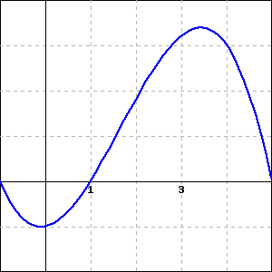
7. Interpreting a graph of $f^{'}$ .

🔗

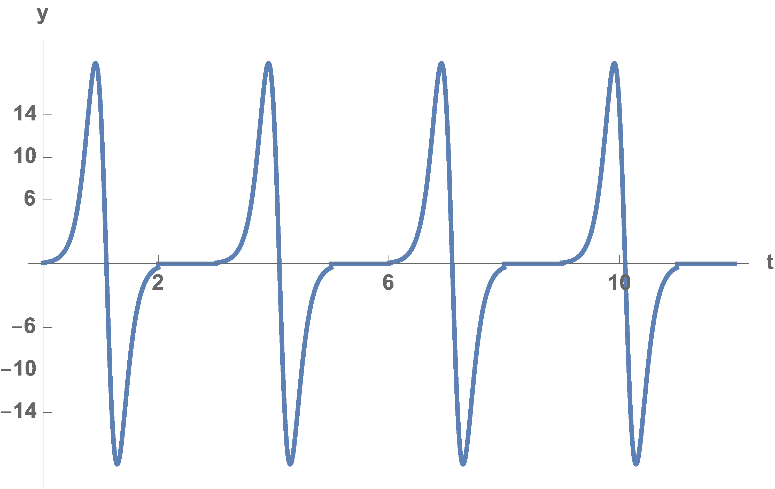
For a certain function

y = g (x),

its derivative is given by the function pictured in Figure 1.95.

Figure 1.95. The graph of $y = g^{'} (x) .$

🔗

What is the approximate slope of the tangent line to $y = g (x)$ at the point $(2, g (2)) ?$
How many real number solutions can there be to the equation $g (x) = 0 ?$ Justify your conclusion fully and carefully by explaining what you know about how the graph of $g$ must behave based on the given graph of $g^{'} .$
On the interval $- 3 < x < 3,$ how many times does the concavity of $g$ change? Why?
Use the provided graph to estimate the value of $g^{″} (2) .$

🔗

8. Using data to interpret derivatives.

🔗

A bungee jumper’s height

h

(in feet ) at time

t

(in seconds) is given in part by the table:

$t$	$0.0$	$0.5$	$1.0$	$1.5$	$2.0$	$2.5$	$3.0$	$3.5$	$4.0$	$4.5$	$5.0$
$h (t)$	$200$	$184.2$	$159.9$	$131.9$	$104.7$	$81.8$	$65.5$	$56.8$	$55.5$	$60.4$	$69.8$

$t$	$5.5$	$6.0$	$6.5$	$7.0$	$7.5$	$8.0$	$8.5$	$9.0$	$9.5$	$10.0$
$h (t)$	$81.6$	$93.7$	$104.4$	$112.6$	$117.7$	$119.4$	$118.2$	$114.8$	$110.0$	$104.7$

🔗

Use the given data to estimate $h^{'} (4.5),$ $h^{'} (5),$ and $h^{'} (5.5) .$ At which of these times is the bungee jumper rising most rapidly?
Use the given data and your work in (a) to estimate $h^{″} (5) .$
What physical property of the bungee jumper does the value of $h^{″} (5)$ measure? What are its units?
Based on the data, on what approximate time intervals is the function $y = h (t)$ concave down? What is happening to the velocity of the bungee jumper on these time intervals?

🔗

9. Sketching functions.

🔗

For each prompt that follows, sketch a possible graph of a function on the interval

- 3 < x < 3

that satisfies the stated properties.

$y = f (x)$ such that $f$ is increasing on $- 3 < x < 3,$ concave up on $- 3 < x < 0,$ and concave down on $0 < x < 3 .$
$y = g (x)$ such that $g$ is increasing on $- 3 < x < 3,$ concave down on $- 3 < x < 0,$ and concave up on $0 < x < 3 .$
$y = h (x)$ such that $h$ is decreasing on $- 3 < x < 3,$ concave up on $- 3 < x < - 1,$ neither concave up nor concave down on $- 1 < x < 1,$ and concave down on $1 < x < 3 .$
$y = p (x)$ such that $p$ is decreasing and concave down on $- 3 < x < 0$ and is increasing and concave down on $0 < x < 3 .$

Prev Top Next

Section 1.7 The Second Derivative

Motivating Questions

Supplemental Videos.

Example 1.76.

Subsection 1.7.1 Increasing, Decreasing, or Neither

Increasing and Decreasing Functions.

Subsection 1.7.2 The Second Derivative

Second Derivative.

Subsection 1.7.3 Concavity

Concavity.

Example 1.86.

Example 1.88.

Example 1.91.

Subsection 1.7.4 Acceleration

Example 1.93.

Subsection 1.7.5 Summary

Exercises 1.7.6 Exercises

1. Comparing f,f′,f″ values.

2. Signs of f,f′,f″ values.

3. Acceleration from velocity.

4. Rates of change of stock values.

5. Interpreting a graph of f′.

6. Interpretting a graph of f based on the first and second derivatives.

7. Interpreting a graph of f′.

8. Using data to interpret derivatives.

9. Sketching functions.

1. Comparing $f, f^{'}, f^{″}$ values.

2. Signs of $f, f^{'}, f^{″}$ values.

5. Interpreting a graph of $f^{'}$ .

6. Interpretting a graph of $f$ based on the first and second derivatives.

7. Interpreting a graph of $f^{'}$ .