Vector Fields

Section4.1Vector Fields

Objectives

What is a vector field?
What are some familiar contexts in which vector fields arise?
How do we draw a vector field?
How do gradients of functions with partial derivatives connect to vector fields?

Thus far vectors have played a central role in our study of multivariable calculus. We know how to do operations on vectors (addition, scalar multiplication, dot product, etc.), and we have seen how vectors can be used to describe curves in $\R^2$ and $\R^3\text{.}$ The examples of using vectors to describe curves was our first example of a vector-valued function. That is, a curve $\vr(t)$ is a function that takes as input a real number and produces a vector in $\R^2$ or $\R^3\text{.}$ In this section, we will expand our understanding of vector-valued functions to take as input a point $(x,y)$ in $\R^2$ or a point $(x,y,z)$ in $\R^3$ and produce a vector (typically in $\R^2$ or $\R^3\text{,}$ respectively).

Exploration4.1.1

It's common for weather forecasters to discuss the wind speed, but as any student who has gotten this far in the text will know, this nomenclature is imprecise. It's not terribly helpful to tell someone the wind is blowing at 10^km_h without telling them the direction in which the wind is blowing. If you're trying to make a decision based on what the wind is doing, you need to know about the direction as well. (Perhaps you are taking off in a hot air balloon and need to know which direction the chase team should head to keep track of you.) Because of the swirling nature of wind, it makes sense to give the wind velocity at every point in a region (two-dimensional or three-dimensional).

(a)

Suppose that given a point $(x,y)$ in the plane, you know that the wind velocity at that point is given by the vector $\vF(x,y) = \langle y,x\rangle\text{.}$ For example, we'd then know that at the point $(1,-1)\text{,}$ the wind velocity is $\vF(1,-1) = \langle -1,1\rangle\text{.}$ In the table below, fill in the wind velocity vectors for the given points.

$(x,y)$	$(2,1)$	$(0,0)$	$(-1,2)$	$(3,-1)$	$(-2,-1)$
$\vF(x,y)$

Solution

The vector field $\vF(x,y)$ takes the coordinates of the point $(x,y)$ and reverses them to make the components of the vector. Thus, $\vF(2,1) = \langle 1,2\rangle\text{.}$ The remaining vectors are shown in the table below.

$(x,y)$	$(2,1)$	$(0,0)$	$(-1,2)$	$(3,-1)$	$(-2,-1)$
$\vF(x,y)$	$\langle 1,2\rangle$	$\langle 0,0\rangle$	$\langle 2,-1\rangle$	$\langle -1,3\rangle$	$\langle -1,-2\rangle$

(b)

Suppose that we associate the vector $\vG(x,y) = -x\vj$ to a point $(x,y)$ in the plane. Complete the table below by giving the vector associated to each of the given points.

$(x,y)$	$(-2,0)$	$(-1,2)$	$(0,-2)$	$(1,1)$	$(2,3)$	$(3,2)$	$(-1,0)$	$(1,3)$
$\vG(x,y)$

Solution

Note that another way of writing $\vG(x,y)$ is $\langle 0 -x\rangle\text{.}$ Thus, $\vG(2,3) = \langle 0,-2\rangle\text{,}$ for example. The remaining answers are found in the table below.

$(x,y)$	$(-2,0)$	$(-1,2)$	$(0,-2)$	$(1,1)$	$(2,3)$	$(3,2)$	$(-1,0)$	$(1,3)$
$\vG(x,y)$	$\langle 0,2\rangle$	$\langle 0,1\rangle$	$\langle 0,0\rangle$	$\langle 0,-1\rangle$	$\langle 0,-2\rangle$	$\langle 0,-3\rangle$	$\langle 0,1\rangle$	$\langle 0,-1\rangle$

(c)

A table of values of these vector-valued functions is useful, but perhaps even better is a method of visualizing the vectors. In keeping with our wind velocity analogy, if $\vF(2,1) = \langle 1,2\rangle\text{,}$ we draw the vector $\langle 1,2\rangle$ with its tail at the point $(2,1)\text{.}$

Using the first set of axes in Figure4.1.1, plot the vectors $\vF(x,y)$ for the five points in the table in parta. The example $\vF(1,-1) = \langle -1,1\rangle$ is drawn for you.

(d)

Using the second set of axes in Figure4.1.1, plot the vectors $\vG(x,y)$ for the eight points in the table in partb.

Axes for a rectangular coordinate system. The horizontal axis is labeled $x$ and the vertical axis is labeled $y\text{.}$ Both axes range from $-4$ to $4\text{.}$ There is a blue vector pointing from the point $(1,-1)$ to the point $(0,0)\text{.}$ — Figure4.1.1Axes for plotting some vectors from $\vF(x,y)$ and $\vG(x,y)\text{.}$

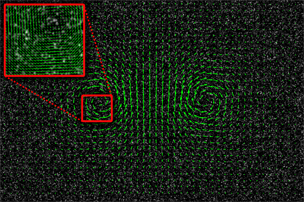
Axes for a rectangular coordinate system. The horizontal axis is labeled $x$ and the vertical axis is labeled $y\text{.}$ Both axes range from $-4$ to $4\text{.}$ — Figure4.1.1Axes for plotting some vectors from $\vF(x,y)$ and $\vG(x,y)\text{.}$

Subsection4.1.1Examples of Vector Fields

As Exploration4.1.1 showed you, a velocity vector field is an example of a scenario where associating a vector to each point in a region is useful. We denote such a vector field by $\vF(x,y)$ or $\vF(x,y,z)\text{,}$ where the vector associated to the point $(x,y)$ or $(x,y,z)$ is the velocity of something at that point. Wind velocity is one example, but another example would be the velocity of a flowing fluid. Figure4.1.2 shows such a velocity vector field. Technically, it only shows some of the vectors in the vector field, since the figure would be unintelligible if all of the vectors were shown. This is illustrated by the inset in the upper left corner, which gives a better picture of what we would see if we zoomed in on the red square of the main figure.

Green vectors representing the velocity vectors of a flowing fluid. The vectors along the vertical axis of symmetry are directed from bottom to top and are longest in the middle. Vectors on either side of the vertical axis of symmetry form circular rotation patterns, clockwise on the right and counterclockwise on the left. In the upper left corner, there is an inset figure that enlarges the center of rotation on the left side of the image. — Figure4.1.2An illustration of some of the vectors in a fluid velocity vector field. "PIVlab multipass" by Willa Licensed under CC-BY-SA 3.0 via Wikimedia Commons.

Force fields, such as those created by gravity, are also examples of vector fields. For example, the earth exerts a gravitational force on objects. The force is directed from the center of the object to the center of the earth, and its magnitude is determined by the distance between the object and the earth. An illustration of this vector field can be seen in Figure4.1.3, where the earth is positioned at the origin, but not shown. Notice that the vectors get shorter as the distance from the origin increases, reflecting the fact that the gravitational force is weaker at that distance.

Figure4.1.3Gravitational vector field.

Subsection4.1.2Mathematical Vector Fields

As suggested in the introduction and Exploration4.1.1, vector fields can be given by formulas.

Definition4.1.4

A vector field in $2$-space is function whose value at a point $(x,y)$ is a $2$-dimensional vector $\vF(x,y)\text{.}$ Similarly, in $3$-space, a vector field is a function $\vF(x,y,z)$ whose value at the point $(x,y,z)$ is a $3$-dimensional vector.

Since $\vF(x,y,z)$ is a vector, it has $\vi\text{,}$ $\vj\text{,}$ and $\vk$ components. Each of these components is a scalar function of the point $(x,y,z)\text{,}$ and so we will often write

\begin{equation*} \vF(x,y,z) = F_1(x,y,z)\vi + F_2(x,y,z)\vj + F_3(x,y,z)\vk\text{.} \end{equation*}

For example, if $\vF(x,y,z) = \langle x^2,xy\sin(z),y^3\rangle\text{,}$ then $F_1(x,y,z) = x^2\text{,}$ $F_2(x,y,z) = xy\sin(z)\text{,}$ and $F_3(x,y,z) = y^3\text{.}$ Any time we are considering a vector field $\vF(x,y,z)\text{,}$ the definitions of functions $F_1\text{,}$ $F_2\text{,}$ and $F_3$ should be assumed in this manner. (For a vector field $\vF(x,y)$ in $2$-space, we only have the functions $F_1$ and $F_2\text{,}$ defined analogously.)

Subsection4.1.3Plotting Vector Fields

Exploration4.1.1 gave you a chance to plot some vectors in the vector fields $\vF(x,y) = \langle y,x\rangle$ and $\vG(x,y) = \langle 0,-x\rangle\text{.}$ It would be impossible to sketch all of the vectors in these vector fields, since there is one for every point in the plane. In fact, even sketching by hand many more of the vectors than you were asked to in the preview activity rapidly becomes tedious. Fortunately, computer algebra systems can do a great job of making such sketches.

One tool to plot 2D vector fields can be found here.

One thing to keep in mind, however, is that the magnitudes of the vectors are typically scaled in these plots, including plots of vector fields we will encounter later in the text. To illustrate this, consider the two plots of the vector field $\vF(x,y) = y\vi + x\vj$ in Figure4.1.5.

A vector field in the plane with both axes ranging from $-2$ to $2\text{.}$ Vectors point from the point $(x,y)$ to the point $(x+y,x+y)\text{.}$ — Figure4.1.5Two plots of $\vF(x,y) = y\vi + x\vj$ from a computer algebra system

A vector field in the plane with both axes ranging from $-2$ to $2\text{.}$ Vectors are shorter closer to the origin and longer farther away. At the left and right sides, the vectors follow arcs oriented clockwise. At the top and right sides, the vectors follow arcs oriented counterclockwise. — Figure4.1.5Two plots of $\vF(x,y) = y\vi + x\vj$ from a computer algebra system

The left plot shows some of the vectors but accurately depicts all of their magnitudes, making the figure very hard to understand, especially along the lines $y=x$ and $y=-x\text{.}$ The plot on the right, however, uses a uniform scaling to make the figure easier to read. As before, each vector's direction is completely accurate, but now the magnitudes are much smaller. However, the relative magnitudes are preserved, helping us to see that vectors farther from the origin have larger magnitude than those closer to the origin.

Example4.1.6

The plot in Figure4.1.7 illustrates the vector field $\vF(x,y) = y\vi -x\vj\text{.}$

A vector field plotted in the plane with $x$ and $y$ both ranging from $-5$ to $5\text{.}$ The vectors have a counterclockwise rotation about the origin, with vectors getting progressively longer as they get farther from the origin. — Figure4.1.7The vector field $y\vi-x\vj$

(a)

Starting with one of the vectors near the point $(2,0)\text{,}$ sketch a curve that follows the direction of the vector field $\vF\text{.}$ To help visualize what you are doing, it may be useful to think of the vector field as the velocity vector field for some flowing water and that you are imagining tracing the path that a tiny particle inserted into the water would follow as the water moved it around.

(b)

Repeat the previous step for at least two other starting points not on the curve you previously sketched.

(c)

What shape do the curves you sketched in the previous two steps form?

(d)

Verify that $\vF(x,y)$ is orthogonal to $\langle x,y\rangle\text{.}$

(e)

What is the relationship between the function $f(x,y) = x^2 + y^2$ and the vector $x\vi + y\vj\text{?}$

(f)

What does this tell you about the relationship between $\vF(x,y)$ and circles centered at the origin? What is the relationship between $\vecmag{\vF(x,y)}$ and the radius of the appropriate circle?

Solution

(a)

$An animated vector field plotted in the plane with $x$ and $y$ both ranging from $-5$ to $5\text{.}$ The vectors have a counterclockwise rotation about the origin, with vectors getting progressively longer as they get farther from the origin. Starting at $(2,0)\text{,}$ the circle of radius $2$ centered at the origin gradually appears.$

(b)

(c)

Circles centered at the origin.

(d)

\begin{equation*} \vF(x,y) \cdot \langle x,y \rangle = \langle y, -x \rangle \cdot \langle x,y \rangle = yx - xy = 0 \end{equation*}

(e)

Notice that the gradient of $f(x,y) = x^2 + y^2$ is $\langle 2x, 2y \rangle\text{,}$ which is a scalar multiple of $\langle x,y \rangle\text{.}$ Therefore $\langle x,y \rangle$ will be orthogonal to the level curves of $f$ (which are circles centered at the origin).

Subsection4.1.4Gradient Vector Fields

Without using the terminology, we've actually already encountered one very important family of vector fields a number of times. Given a function $f$ of two or three variables, the gradient of $f$ is a vector field, since for any point where $f$ has first-order partial derivatives, $\grad{f}$ assigns a vector to that point.

Activity4.1.2

(a)

In Figure4.1.8 there are three sets of axes showing level curves for functions $f\text{,}$ $g\text{,}$ and $h\text{,}$ respectively. Sketch at least six vectors in the gradient vector field for each function. In making your sketches, you don't have to worry about getting vector magnitudes precise, but you should ensure that the relative magnitudes (and directions) are correct for each function independently.

Eight skew ellipses centered at the origin. The major axis of the ellipses is the line $y=-x\text{.}$ Labels on the ellipses range from $25$ to $200$ in increments of $25\text{.}$ The axes range approximately from $-8$ to $8\text{.}$ — (a)$f$

Seven equally-spaced lines with slope $1/2$ plotted on axes that range approximately from $-8$ to $8\text{.}$ The lines are labeled from $-60$ to $60$ increments of $20\text{.}$ — (a)$f$

(b)

Verify that $\vF(x,y) = \langle 6xy,3x^2+9\sqrt{y}\rangle$ is a gradient vector field by finding a function $f$ such that $\nabla f(x,y) = \vF(x,y)\text{.}$ For reasons originating in physics, such a function $f$ is called a potential function for the vector field $\vF\text{.}$

(c)

Is the function $f$ found in partb unique? That is, can you find another function $g$ such that $\nabla g(x,y) = \vF(x,y)$ but $f\neq g\text{?}$

(d)

Is the vector field $\vF(x,y) = 6xy\vi +(2x+9\sqrt{y})\vj$ a gradient vector field? Why or why not?

Subsection4.1.5Summary

A $2$-dimensional vector field is a function defined on part of $\R^2$ whose value is a $2$-dimensional vector. A $3$-dimensional vector field is a function defined on part of $\R^3$ whose value is a $3$-dimensional vector.
Vector fields arise in familiar contexts such as wind velocity, fluid velocity, and gravitational force.
Vector fields are generally plotted in ways that ensure the direction and relative magnitudes of the vectors sketched are correct instead of ensuring that each vector's magnitude is depicted correctly.
The gradient of a function $f$ of two or three variables is a vector field defined wherever $f$ has partial derivatives.

Subsection4.1.6Exercises

1

Match the formulas with the corresponding vector field plots.

$\vi$
$\vj$
$x \vi$
$x \vj$
$y \vi$
$y \vj$

Hint

In a vector field of the form $k \vi$ where $k$ is a scalar (e.g. $k=1$ or $k=x$ or $k = y$), all the vectors must be horizontal. Likewise, in a vector field of the form $k \vj$ all vectors must be vertical. Consider the lengths of the vectors, too.

2

In the two images below you'll see contour maps for two different functions. On each contour map, draw the gradient field of the function.

(a)

(b)

Figure4.1.10

Hint

The gradient vector is always orthogonal to the contour line, it points in the direction of greatest ascent, and its length is the directional derivative in the direction of greatest ascent. Don't forget that the function is changing most rapidly where the contour lines are closest together.

Solution

(a)

(b)

Figure4.1.11

\((x,y)\)	\((2,1)\)	\((0,0)\)	\((-1,2)\)	\((3,-1)\)	\((-2,-1)\)
\(\vF(x,y)\)

\((x,y)\)	\((2,1)\)	\((0,0)\)	\((-1,2)\)	\((3,-1)\)	\((-2,-1)\)
\(\vF(x,y)\)	\(\langle 1,2\rangle\)	\(\langle 0,0\rangle\)	\(\langle 2,-1\rangle\)	\(\langle -1,3\rangle\)	\(\langle -1,-2\rangle\)

\((x,y)\)	\((-2,0)\)	\((-1,2)\)	\((0,-2)\)	\((1,1)\)	\((2,3)\)	\((3,2)\)	\((-1,0)\)	\((1,3)\)
\(\vG(x,y)\)

\((x,y)\)	\((-2,0)\)	\((-1,2)\)	\((0,-2)\)	\((1,1)\)	\((2,3)\)	\((3,2)\)	\((-1,0)\)	\((1,3)\)
\(\vG(x,y)\)	\(\langle 0,2\rangle\)	\(\langle 0,1\rangle\)	\(\langle 0,0\rangle\)	\(\langle 0,-1\rangle\)	\(\langle 0,-2\rangle\)	\(\langle 0,-3\rangle\)	\(\langle 0,1\rangle\)	\(\langle 0,-1\rangle\)