Optimization

Section 2.6 Optimization

Motivating Questions

How can we find the points at which $f(x,y)$ has a local maximum or minimum?
How can we determine whether critical points of $f(x,y)$ are local maxima or minima?
How can we find the absolute maximum and minimum of $f(x,y)$ on a closed and bounded domain?

We learn in single-variable calculus that the derivative is a useful tool for finding the local maxima and minima of functions, and that these ideas may often be employed in applied settings. In particular, if a function $f\text{,}$ such as the one shown in Figure 2.6.1 is everywhere differentiable, we know that the tangent line is horizontal at any point where $f$ has a local maximum or minimum. This, of course, means that the derivative $f'$ is zero at any such point. Hence, one way that we seek extreme values of a given function is to first find where the derivative of the function is zero.

Figure 2.6.1. The graph of $y=f(x)\text{.}$

In multivariable calculus, we are often similarly interested in finding the greatest and/or least value(s) that a function may achieve. Moreover, there are many applied settings in which a quantity of interest depends on several different variables. In the following preview activity, we begin to see how some key ideas in multivariable calculus can help us answer such questions by thinking about the geometry of the surface generated by a function of two variables.

Preview Activity 2.6.1.

Let $z = f(x,y)$ be a differentiable function, and suppose that at the point $(x_0, y_0)\text{,}$ $f$ achieves a local maximum. That is, the value of $f(x_0,y_0)$ is greater than the value of $f(x,y)$ for all $(x,y)$ nearby $(x_0,y_0)\text{.}$ You might find it helpful to sketch a rough picture of a possible function $f$ that has this property.

If we consider the trace given by holding $y=y_0$ constant, then the single-variable function defined by $f(x, y_0)$ must have a local maximum at $x_0\text{.}$ What does this say about the value of the partial derivative $f_x(x_0,y_0)\text{?}$
In the same way, the trace given by holding $x=x_0$ constant has a local maximum at $y=y_0\text{.}$ What does this say about the value of the partial derivative $f_y(x_0,y_0)\text{?}$
What may we now conclude about the gradient $\nabla f(x_0,y_0)$ at the local maximum? How is this consistent with the statement “$f$ increases most rapidly in the direction $\nabla f(x_0,y_0)\text{?}$”
How will the tangent plane to the surface $z = f(x,y)$ appear at the point $(x_0, y_0, f(x_0,y_0))\text{?}$
By first computing the partial derivatives, find any points at which $f(x,y) = 2x - x^2 - (y + 2)^2$ may have a local maximum.

Subsection 2.6.1 Extrema and Critical Points

One of the important applications of single-variable calculus is the use of derivatives to identify local extremes of functions (that is, local maxima and local minima). Using the tools we have developed so far, we can naturally extend the concept of local maxima and minima to several-variable functions.

Definition 2.6.2.

Let $f$ be a function of two variables $x$ and $y\text{.}$

The function $f$ has a local maximum at a point $(x_0,y_0)$ provided that $f(x,y) \leq f(x_0,y_0)$ for all points $(x,y)$ near $(x_0,y_0)\text{.}$ In this situation we say that $f(x_0, y_0)$ is a local maximum value.
The function $f$ has a local minimum at a point $(x_0,y_0)$ provided that $f(x,y) \geq f(x_0,y_0)$ for all points $(x,y)$ near $(x_0,y_0)\text{.}$ In this situation we say that $f(x_0, y_0)$ is a local minimum value.
An absolute maximum point is a point $(x_0,y_0)$ for which $f(x,y)\leq f(x_0,y_0)$ for all points $(x,y)$ in the domain of $f\text{.}$ The value of $f$ at an absolute maximum point is the maximum value of $f\text{.}$
An absolute minimum point is a point such that $f(x,y) \geq f(x_0,y_0)$ for all points $(x,y)$ in the domain of $f\text{.}$ The value of $f$ at an absolute minimum point is the minimum value of $f\text{.}$

We use the term extremum point to refer to any point $(x_0,y_0)$ at which $f$ has a local maximum or minimum. In addition, the function value $f(x_0,y_0)$ at an extremum is called an extremal value. Figure 2.6.3 illustrates the graphs of two functions that have an absolute maximum and minimum, respectively, at the origin $(x_0,y_0) = (0,0)\text{.}$

Figure 2.6.3. An absolute maximum and an absolute minimum

In single-variable calculus, we saw that the extrema of a continuous function $f$ always occur at critical points, values of $x$ where $f$ fails to be differentiable or where $f'(x) = 0\text{.}$ Said differently, critical points provide the locations where extrema of a function may appear. Our work in Preview Activity 2.6.1 suggests that something similar happens with two-variable functions.

Suppose that a continuous function $f$ has an extremum at $(x_0,y_0)\text{.}$ In this case, the trace $f(x,y_0)$ has an extremum at $x_0\text{,}$ which means that $x_0$ is a critical value of $f(x,y_0)\text{.}$ Therefore, either $f_x(x_0,y_0)$ does not exist or $f_x(x_0,y_0) = 0\text{.}$ Similarly, either $f_y(x_0,y_0)$ does not exist or $f_y(x_0,y_0) = 0\text{.}$ This implies that the extrema of a two-variable function occur at points that satisfy the following definition.

Definition 2.6.4.

A critical point $(x_0,y_0)$ of a function $f=f(x,y)$ is a point in the domain of $f$ at which $f_x(x_0,y_0) = 0$ and $f_y(x_0,y_0) = 0\text{,}$ or such that one of $f_x(x_0,y_0)$ or $f_y(x_0,y_0)$ fails to exist.

We can therefore find critical points of a function $f$ by computing partial derivatives and identifying any values of $(x,y)$ for which one of the partials doesn’t exist or for which both partial derivatives are simultaneously zero. For the latter, note that we have to solve the system of equations

\begin{align*} f_x(x,y) \amp = 0\\ f_y(x,y) \amp = 0. \end{align*}

Activity 2.6.2.

Find the critical points of each of the following functions. Then, using appropriate technology, plot the graphs of the surfaces near each critical point and compare the graph to your work.

$\displaystyle f(x,y) = 2+x^2+y^2$
$\displaystyle f(x,y) = 2 + x^2 - y^2$
$\displaystyle f(x,y) = 2x-x^2-\frac{1}{4}y^2$
$\displaystyle f(x,y) = |x| + |y|$
$f(x,y) = 2xy - 4x + 2y - 3\text{.}$

Answer.

The only critical point of $f$ is at $(0,0)\text{.}$

The partial derivatives of $f$ are $f_x(x,y) = 2x$ and $f_y(x,y) = 2y\text{.}$ Both partial derivatives are defined everywhere so we only need to solve the system of equations

\begin{align*} 2x \amp = 0\\ 2y \amp = 0, \end{align*}

which has a unique solution at $(0,0)\text{.}$
The only critical point of $f$ is at $(0,0)\text{.}$

The partial derivatives of $f$ are $f_x(x,y) = 2x$ and $f_y(x,y) = -2y\text{.}$ Both partial derivatives are defined everywhere so we only need to solve the system of equations

\begin{align*} 2x \amp = 0\\ -2y \amp = 0, \end{align*}

which also has a unique solution at $(0,0)\text{.}$
The only critical point of $f$ is at $(1,0)\text{.}$

The partial derivatives of $f$ are $f_x(x,y) = 2 - 2x$ and $f_y(x,y) = -\frac{1}{2}y\text{.}$ Both partial derivatives are defined everywhere so we only need to solve the system of equations

\begin{align*} 2-2x \amp = 0\\ -\frac{1}{2}y \amp = 0, \end{align*}

which also has a unique solution at $(1,0)\text{.}$
The critical points of $f$ are of the form $(0,y)$ for any real $y$ and $(x,0)$ for any real $x\text{.}$

Recall from calculus 1 that $|x|$ is undefined when $x=0$ since it has a slope of $-1$ to the left of 0 and a slope of $1$ to the right of 0. Similarly, $f(x,y) = |x| + |y|$ fails to have a partial derivative in the $x$-direction when $x=0$ and fails to have a partial derivative in the $y$-direction when $y=0\text{.}$ We then have an infinitely many critical points caused by partials failing to exist: points of the form $(0,y)$ for any real $y$ and $(x,0)$ for any real $x\text{.}$ On the othe hand, when the partial derivatives are defined in either direction they will always be 1 or -1, and never 0, so we have no critical points caused by the partials equalling 0.
The only critical point of $f$ is at $(-1,2)\text{.}$

The partial derivatives of $f$ are $f_x(x,y) = 2y - 4$ and $f_y(x,y) = 2x + 2\text{.}$ Both partial derivatives are defined everywhere so we only need to solve the system of equations

\begin{align*} 2y - 4 \amp = 0\\ 2x + 2 \amp = 0, \end{align*}

which also has a unique solution at $(-1,2)\text{.}$

Subsection 2.6.2 Classifying Critical Points: The Second Derivative Test

While the extrema of a continuous function $f$ always occur at critical points, it is important to note that not every critical point leads to an extremum. Recall, for instance, $f(x) = x^3$ from single variable calculus. We know that $x_0=0$ is a critical point since $f'(x_0) = 0\text{,}$ but $x_0 = 0$ is neither a local maximum nor a local minimum of $f\text{.}$

A similar situation may arise in a multivariable setting. Consider the function $f$ defined by $f(x,y) = x^2 - y^2$ whose graph and contour plot are shown in Figure 2.6.5. Because $\nabla f = \langle 2x, -2y\rangle\text{,}$ we see that the origin $(x_0,y_0)=(0,0)$ is a critical point. However, this critical point is neither a local maximum or minimum; the origin is a local minimum on the trace defined by $y=0\text{,}$ while the origin is a local maximum on the trace defined by $x=0\text{.}$ We call such a critical point a saddle point due to the shape of the graph near the critical point.

As in single-variable calculus, we would like to have some sort of test to help us identify whether a critical point is a local maximum, local maximum, or neither.

Activity 2.6.3.

Recall that the Second Derivative Test for single-variable functions states that if $x_0$ is a critical point of a function $f$ so that $f'(x_0)=0$ and if $f''(x_0)$ exists, then

if $f''(x_0) \lt 0\text{,}$ $x_0$ is a local maximum,
if $f''(x_0) > 0\text{,}$ $x_0$ is a local minimum, and
if $f''(x_0) = 0\text{,}$ this test yields no information.

Our goal in this activity is to understand a similar test for classifying extreme values of functions of two variables. Consider the following three functions:

\begin{equation*} f_1(x,y) = 4-x^2-y^2, \ \ f_2(x,y) = x^2+y^2, \ \ f_3(x,y) = x^2-y^2. \end{equation*}

You can verify that each function has a critical point at the origin $(0,0)\text{.}$ You should check this.

The graphs of these three functions are shown in Figure 2.6.6, with $z=4-x^2-y^2$ at left, $z=x^2+y^2$ in the middle, and $z=x^2-y^2$ at right. Use the graphs to decide if a function has a local maximum, local minimum, saddle point, or none of the above at the origin.
There is no single second derivative of a function of two variables, so we consider a quantity that combines the second order partial derivatives. Let $D = f_{xx}f_{yy} - f_{xy}^2\text{.}$ Calculate $D$ at the origin for each of the functions $f_1\text{,}$ $f_2\text{,}$ and $f_3\text{.}$ What difference do you notice between the values of $D$ when a function has a maximum or minimum value at the origin versus when a function has a saddle point at the origin?
Now consider the cases where $D \gt 0\text{.}$ It is in these cases that a function has a local maximum or minimum at a point. What is necessary in these cases is to find a condition that will distinguish between a maximum and a minimum. In the cases where $D \gt 0$ at the origin, evaluate $f_{xx}(0,0)\text{.}$ What value does $f_{xx}(0,0)$ have when $f$ has a local maximum value at the origin? When $f$ has a local minimum value at the origin? Explain why. (Hint: This should look very similar to the Second Derivative Test for functions of a single variable.) What would happen if we considered the values of $f_{yy}(0,0)$ instead?

Answer.

The function $f_1(x,y)=4-x^2-y^2$ has a local maximum at the origin, $f_2(x,y)=x^2+y^2$ has a local minimum at the origin, and $f_3(x,y)=x^2-y^2$ has a saddle point at the origin.
For $f_1(x,y)=4-x^2-y^2\text{,}$ the first and second partial derivatives are

\begin{align*} f_x(x,y) \amp = -2x\\ f_y(x,y) \amp = -2y\\ f_{xx}(x,y) \amp = -2\\ f_{xy}(x,y) \amp = 0\\ f_{yy}(x,y) \amp = -2 \end{align*}

so at $(0,0)$ we get

\begin{align*} D \amp = f_{xx}(0,0)f_{yy}(0,0)-(f_{xy}(0,0))^2\\ \amp = (-2)(-2)-(0)^2 =4. \end{align*}

For $f_2(x,y)=x^2+y^2\text{,}$ the first and second partial derivatives are

\begin{align*} f_x(x,y) \amp = 2x\\ f_y(x,y) \amp = 2y\\ f_{xx}(x,y) \amp = 2\\ f_{xy}(x,y) \amp = 0\\ f_{yy}(x,y) \amp = 2 \end{align*}

so at $(0,0)$ we get

\begin{align*} D \amp = f_{xx}(0,0)f_{yy}(0,0)-(f_{xy}(0,0))^2\\ \amp = (2)(2)-(0)^2 =4. \end{align*}

For $f_3(x,y)=x^2-y^2\text{,}$ the first and second partial derivatives are

\begin{align*} f_x(x,y) \amp = 2x\\ f_y(x,y) \amp = -2y\\ f_{xx}(x,y) \amp = 2\\ f_{xy}(x,y) \amp = 0\\ f_{yy}(x,y) \amp = -2 \end{align*}

so at $(0,0)$ we get

\begin{align*} D \amp = f_{xx}(0,0)f_{yy}(0,0)-(f_{xy}(0,0))^2\\ \amp = (2)(-2)-(0)^2 =-4. \end{align*}

We can see that $D$ is positive at the origin for the maximum and minimum examples and negative at the origin for the saddle point example.
From our calculations above, we get that $f_{xx}(0,0)\lt 0$ for a local maximum and $f_{xx}(0,0)\gt 0$ for a local minimum. We also get that $f_{yy}(0,0)\lt 0$ for a local maximum and $f_{yy}(0,0)\gt 0$ for a local minimum.

Activity 2.6.3 provides the basic ideas for the Second Derivative Test for functions of two variables.

The Second Derivative Test.

Suppose $(x_0,y_0)$ is a critical point of the function $f$ for which $f_x(x_0,y_0) = 0$ and $f_y(x_0,y_0) = 0\text{.}$ Let $D$ be the quantity defined by

\begin{equation*} D = f_{xx}(x_0,y_0) f_{yy}(x_0,y_0) - f_{xy}(x_0,y_0)^2. \end{equation*}

If $D>0$ and $f_{xx}(x_0,y_0) \lt 0\text{,}$ then $f$ has a local maximum at $(x_0,y_0)\text{.}$
If $D>0$ and $f_{xx}(x_0,y_0) > 0\text{,}$ then $f$ has a local minimum at $(x_0,y_0)\text{.}$
If $D \lt 0\text{,}$ then $f$ has a saddle point at $(x_0,y_0)\text{.}$
If $D = 0\text{,}$ then this test yields no information about what happens at $(x_0,y_0)\text{.}$

The quantity $D$ is called the discriminant of the function $f$ at $(x_0,y_0)\text{.}$

To properly understand the origin of the Second Derivative Test, we could introduce a “second-order directional derivative.” If this second-order directional derivative were negative in every direction, for instance, we could guarantee that the critical point is a local maximum. A complete justification of the Second Derivative Test requires key ideas from linear algebra that are beyond the scope of this course, so instead of presenting a detailed explanation, we will accept this test as stated. In Activity 2.6.4, we apply the test to more complicated examples.

Activity 2.6.4.

Find the critical points of the following functions and use the Second Derivative Test to classify the critical points.

$\displaystyle f(x,y) = 3x^3+y^2-9x+4y$
$\displaystyle f(x,y) = xy + \frac{2}{x} + \frac{4}{y}$
$f(x,y) = x^3 + y^3 - 3xy\text{.}$

Answer.

The first derivatives of $f$ are

\begin{align*} f_x(x,y) \amp= 9x^2-9\\ f_y(x,y) \amp= 2y+4 \end{align*}

and both are defined everywhere. We can then find critical points by solving the system of equations

\begin{align*} 9x^2-9 \amp= 0\\ 2y+4 \amp= 0. \end{align*}

We can rewrite $9x^2-9=0$ to $x^2=1\text{,}$ so it must be that $x=\pm 1\text{.}$ From $2y+4=0$ we know $y= -2\text{.}$ We then get two critical points: $(1,-2)$ and $(-1,-2)\text{.}$

The second derivatives of $f$ are

\begin{align*} f_{xx}(x,y) \amp= 18x\\ f_{xy}(x,y) \amp= 0\\ f_{yy}(x,y) \amp= 2 \end{align*}

so the determinant at $(x,y)$ is

\begin{equation*} D=36x. \end{equation*}

Then at $(1,-2)$ the determinant is $D=36\gt 0$ and $f_{xx}(1,-2) =18\gt 0\text{,}$ so $f$ has a local minimum at $(1,-2)\text{.}$ On the other hand, at $(-1,-2)$ the determinant is $D=-36\lt 0\text{,}$ so $f$ has a saddle point at $(1,-2)\text{.}$
The first derivatives of $f$ are

\begin{align*} f_x(x,y) \amp= y - \frac{2}{x^2}\\ f_y(x,y) \amp= x - \frac{4}{y^2}. \end{align*}

The partial in the $x$-direction is then undefined when $x=0$ and the partial in the $y$-direction is undefined when $y=0\text{.}$ Any point of the form $(0,y)$ or $(x,0)$ where $x$ and $y$ are real numbers is then a critical point of $f\text{.}$ For critical points caused by both partials being zero, we solve the system of equations

\begin{align*} y - \frac{2}{x^2} \amp= 0\\ x - \frac{4}{y^2} \amp= 0. \end{align*}

Note that if both partials are zero we’re implicitly assuming that they’re both defined, so in particular we’re assuming that $x\neq 0$ and $y\neq 0\text{.}$ We can rewrite $y - \frac{2}{x^2}=0$ to $y = \frac{2}{x^2}$ then $y^2 = \frac{4}{x^4}\text{,}$ so $x^4 = \frac{4}{y^2}\text{.}$ Now we can substitute that back in to $x - \frac{4}{y^2}=0$ to get $x(1-x^3) = x - x^4=0$ which has solutions when $x=0$ and $x=1\text{.}$ However, we’ve already assumed $x\neq 0\text{,}$ so we just get $x=1\text{.}$ Putting $x=1$ back in to $y = \frac{2}{x^2}$ we get $y = 2\text{.}$ We then get one critical point: $(1,2)\text{.}$

The second derivatives of $f$ are

\begin{align*} f_{xx}(x,y) \amp= \frac{4}{x^3}\\ f_{xy}(x,y) \amp= 1\\ f_{yy}(x,y) \amp= \frac{8}{y^3} \end{align*}

so the determinant at $(x,y)$ is

\begin{equation*} D=\left(\frac{4}{x^3}\right)\left(\frac{8}{y^3}\right)-1^2 = \frac{32}{(xy)^3}-1. \end{equation*}

Then at $(1,2)$ the determinant is $D=4\gt 0$ and $f_{xx}(1,2) =4\gt 0\text{,}$ so $f$ has a local minimum at $(1,2)\text{.}$
The first derivatives of $f$ are

\begin{align*} f_x(x,y) \amp= 3x^2 - 3y\\ f_y(x,y) \amp= 3y^2 - 3x \end{align*}

and both are defined everywhere. We can then find critical points by solving the system of equations

\begin{align*} 3x^2 - 3y \amp= 0\\ 3y^2 - 3x \amp= 0. \end{align*}

We can rewrite $3x^2 - 3y=0$ to $x^2=y\text{,}$ so $x^4=y^2\text{.}$ We can then substitute this into the second equation rewritten to $y^2-x=0$ to get $x(x^3-1)=x^4-x=0\text{,}$ which has solutions at $x=0$ and $x=1\text{.}$ Plugging these back in to $x^2=y\text{,}$ we get the two critical points $(0,0)$ and $(1,1)\text{.}$

The second derivatives of $f$ are

\begin{align*} f_{xx}(x,y) \amp= 6x\\ f_{xy}(x,y) \amp= - 3\\ f_{yy}(x,y) \amp= 6y \end{align*}

so the determinant at $(x,y)$ is

\begin{equation*} D=36xy - (-3)^2 = 36xy - 9. \end{equation*}

Then at $(0,0)$ the determinant is $D=-9\lt 0$ so $f$ has a saddle point at $(0,0)\text{.}$ At $(1,1)$ the determinant is $D=27\gt 0$ and $f_{xx}(1,1) =6\gt 0$ so $f$ has a local minimum at $(1,1)\text{.}$

As we learned in single-variable calculus, finding extremal values of functions can be particularly useful in applied settings. For instance, we can often use calculus to determine the least expensive way to construct something or to find the most efficient route between two locations. The same possibility holds in settings with two or more variables.

Activity 2.6.5.

While the quantity of a product demanded by consumers is often a function of the price of the product, the demand for a product may also depend on the price of other products. For instance, the demand for blue jeans at Old Navy may be affected not only by the price of the jeans themselves, but also by the price of khakis.

Suppose we have two goods whose respective prices are $p_1$ and $p_2\text{.}$ The demand for these goods, $q_1$ and $q_2\text{,}$ depend on the prices as

\begin{align} q_1 \amp = 150 - 2p_1 - p_2\tag{2.6.1}\\ q_2 \amp = 200 - p_1 - 3p_2.\tag{2.6.2} \end{align}

The seller would like to set the prices $p_1$ and $p_2$ in order to maximize revenue. We will assume that the seller meets the full demand for each product. Thus, if we let $R$ be the revenue obtained by selling $q_1$ items of the first good at price $p_1$ per item and $q_2$ items of the second good at price $p_2$ per item, we have

\begin{equation*} R = p_1q_1 + p_2q_2. \end{equation*}

We can then write the revenue as a function of just the two variables $p_1$ and $p_2$ by using Equations (2.6.1) and (2.6.2), giving us

\begin{align*} R(p_1,p_2) \amp = p_1(150 - 2p_1 - p_2) + p_2(200 - p_1 - 3p_2)\\ \amp = 150p_1 + 200p_2 - 2p_1p_2 -2p_1^2 - 3p_2^2. \end{align*}

A graph of $R$ as a function of $p_1$ and $p_2$ is shown in Figure 2.6.7.

Find all critical points of the revenue function, $R\text{.}$ (Hint: You should obtain a system of two equations in two unknowns which can be solved by elimination or substitution.)
Apply the Second Derivative Test to determine the type of any critical point(s).
Where should the seller set the prices $p_1$ and $p_2$ to maximize the revenue?

Answer.

The first partial derivatives of $R$ are

\begin{align*} R_{p_1}(p_1,p_2) \amp = 150 - 2p_2 -4p_1\\ R_{p_2}(p_1,p_2) \amp = 200 - 2p_1 -6p_2, \end{align*}

both of which are defined everywhere. We can then find critical points by solving the system of equations

\begin{align*} 150 - 2p_2 -4p_1 \amp = 0\\ 200 - 2p_1 -6p_2 \amp = 0 \end{align*}

which has a critical point at $(25,25)\text{.}$
The second partial derivatives of $R$ are

\begin{align*} R_{p_1p_1}(p_1,p_2) \amp = -4\\ R_{p_1p_2}(p_1,p_2) \amp = - 2\\ R_{p_2p_2}(p_1,p_2) \amp = -6 \end{align*}

so the descriminant of $f$ at $(x,y)$ is

\begin{equation*} D = (-4)(-6)-(-2)^2=20. \end{equation*}

At our critical point $(25,25)$ we then get $D=20\gt 0$ and $R_{p_1p_1}(25,25)=-4\lt 0 \text{,}$ so $f$ has a local minimum at $(25,25)\text{.}$
The seller should set the prices of both $p_1$ and $p_2$ at 25 to maximize the revenue.

Subsection 2.6.3 Optimization on a Restricted Domain

The Second Derivative Test helps us classify critical points of a function, but it does not tell us if the function actually has an absolute maximum or minimum at each such point. For single-variable functions, the Extreme Value Theorem told us that a continuous function on a closed interval $[a, b]$ always has both an absolute maximum and minimum on that interval, and that these absolute extremes must occur at either an endpoint or at a critical point. Thus, to find the absolute maximum and minimum, we determine the critical points in the interval and then evaluate the function at these critical points and at the endpoints of the interval. A similar approach works for functions of two variables.

For functions of two variables, closed and bounded regions play the role that closed intervals did for functions of a single variable. A closed region is a region that contains its boundary (the unit disk $x^2+y^2 \leq 1$ is closed, while its interior $x^2+y^2 \lt 1$ is not, for example), while a bounded region is one that does not stretch to infinity in any direction. Just as for functions of a single variable, continuous functions of several variables that are defined on closed, bounded regions must have absolute maxima and minima in those regions.

The Extreme Value Theorem.

Let $f= f(x,y)$ be a continuous function on a closed and bounded region $R\text{.}$ Then $f$ has an absolute maximum and an absolute minimum in $R\text{.}$

The absolute extremes must occur at either a critical point in the interior of $R$ or at a boundary point of $R\text{.}$ We therefore must test both possibilities, as we demonstrate in the following example.

Example 2.6.8.

Suppose the temperature $T$ at each point on the circular plate $x^2+y^2 \leq 1$ is given by

\begin{equation*} T(x,y) = 2x^2+y^2-y. \end{equation*}

The domain $R=\{(x,y):x^2+y^2 \leq 1\}$ is a closed and bounded region, as shown on the left of Figure 2.6.9, so the Extreme Value Theorem assures us that $T$ has an absolute maximum and minimum on the plate. The graph of $T$ over its domain $R$ is shown in Figure 2.6.9. We will find the hottest and coldest points on the plate.

Figure 2.6.9. Domain of the temperature $T(x,y) = 2x^2+y^2-y$ and its graph.

If the absolute maximum or minimum occurs inside the disk, it will be at a critical point so we begin by looking for critical points inside the disk. To do this, notice that critical points are given by the conditions $T_x= 4x=0$ and $T_y=2y - 1=0\text{.}$ This means that there is one critical point of the function at the point $(x_0,y_0) =(0,1/2)\text{,}$ which lies inside the disk.

We now find the hottest and coldest points on the boundary of the disk, which is the circle of radius 1. As we have seen, the points on the unit circle can be parametrized as

\begin{equation*} x(t) = \cos(t), \ y(t) = \sin(t), \end{equation*}

where $0\leq t \leq 2\pi\text{.}$ The temperature at a point on the circle is then described by

\begin{equation*} T(x(t), y(t)) = 2\cos^2(t) + \sin^2(t) - \sin(t). \end{equation*}

To find the hottest and coldest points on the boundary, we look for the critical points of this single-variable function on the interval $0\leq t\leq 2\pi\text{.}$ We have

\begin{align*} \frac{dT}{dt} \amp = -4\cos(t)\sin(t) + 2\cos(t)\sin(t) -\cos(t)\\ \amp = -2\cos(t)\sin(t) - \cos(t) = \cos(t) (-2\sin(t) - 1)\\ \amp = 0. \end{align*}

This shows that we have critical points when $\cos(t) = 0$ or $\sin(t) = -1/2\text{.}$ This occurs when $t=\pi/2\text{,}$ $3\pi/2\text{,}$ $7\pi/6\text{,}$ and $11\pi/6\text{.}$ Since we have $x(t) = \cos(t)$ and $y(t) = \sin(t)\text{,}$ the corresponding points are

$\bullet\ \ (x,y) = (0,1)$ when $t = \frac{\pi}{2}\text{,}$

$\bullet\ \ (x,y) = \left(\frac{\sqrt{3}}{2},-\frac{1}{2}\right)$ when $t = \frac{11\pi}{6}\text{.}$

$\bullet\ \ (x,y) = (0,-1)$ when $t = \frac{3\pi}{2}\text{,}$

$\bullet\ \ (x,y) = \left(-\frac{\sqrt{3}}{2},-\frac{1}{2}\right)$ when $t = \frac{7\pi}{6}\text{.}$

These are the critical points of $T$ on the boundary and so this collection of points includes the hottest and coldest points on the boundary.

We now have a list of candidates for the hottest and coldest points: the critical point in the interior of the disk and the critical points on the boundary. We find the hottest and coldest points by evaluating the temperature at each of these points, and find that

$\bullet\ \ T\left(0,\frac{1}{2}\right) = -\frac{1}{4}\text{,}$

$\bullet\ \ T\left(-\frac{\sqrt{3}}{2},-\frac{1}{2}\right) = \frac{9}{4}\text{,}$

$\bullet\ \ T\left(0,1\right) = 0\text{,}$

$\bullet\ \ T\left(-\frac{\sqrt{3}}{2},-\frac{1}{2}\right) = \frac{9}{4}\text{.}$

$\bullet\ \ T\left(0,-1\right) = 2\text{,}$

So the maximum value of $T$ on the disk $x^2+y^2\leq 1$ is $\frac{9}{4}\text{,}$ which occurs at the two points $\left(\pm\frac{\sqrt{3}}{2},-\frac{1}{2}\right)$ on the boundary, and the minimum value of $T$ on the disk is $-\frac{1}{4}$ which occurs at the critical point $\left(0,\frac{1}{2}\right)$ in the interior of $R\text{.}$

From this example, we see that we use the following procedure for determining the absolute maximum and absolute minimum of a function on a closed and bounded domain.

Step 1:.
Find all critical points of the function in the interior of the domain.
Step 2:.
Find all the critical points of the function on the boundary of the domain. Working on the boundary of the domain reduces this part of the problem to one or more single variable optimization problems. Note that there may be endpoints on portions of the boundary that need to be considered.
Step 3:.
Evaluate the function at each of the points found in Steps 1 and 2.
Step 4:.
The maximum value of the function is the largest value obtained in Step 3, and the minimum value of the function is the smallest value obtained in Step 3.

Activity 2.6.6.

Let $f(x,y) = x^2-3y^2-4x+6y$ with triangular domain $R$ whose vertices are at $(0,0)\text{,}$ $(4,0)\text{,}$ and $(0,4)\text{.}$ The domain $R$ and a graph of $f$ on the domain appear in Figure 2.6.10.

Figure 2.6.10. The domain of $f(x,y) = x^2-3y^2-4x+6y$ and its graph.

Find all of the critical points of $f$ in $R\text{.}$
Parameterize the horizontal leg of the triangular domain, and find the critical points of $f$ on that leg. (Hint: You may need to consider endpoints.)
Parameterize the vertical leg of the triangular domain, and find the critical points of $f$ on that leg. (Hint: You may need to consider endpoints.)
Parameterize the hypotenuse of the triangular domain, and find the critical points of $f$ on the hypotenuse. (Hint: You may need to consider endpoints.)
Find the absolute maximum and absolute minimum values of $f$ on $R\text{.}$

Answer.

The first partial derivatives of $f$ are

\begin{align*} f_x(x,y) \amp= 2x-4\\ f_y(x,y) \amp= -6y +6, \end{align*}

both of which are defined over all of $R\text{.}$ We can then find critical points for $f$ by solving the system of equations

\begin{align*} 2x-4 \amp= 0\\ -6y +6 \amp= 0 \end{align*}

and identifying the solutions which are in $R\text{.}$ There is a unique solution to the system of equations at the point $(2,1)\text{,}$ which is in $R\text{.}$ Thus the only critical point of $f$ in $R$ is $(2,1)\text{.}$
We can think of the horizontal leg of the triangular domain as the line which starts at the origin and moves one step in the direction $\langle 4,0\rangle\text{.}$ This is parameterized by $\vr(t) = \langle 4t,0\rangle$ for $0\leq t\leq 1\text{.}$ Plugging this parameterization in to $f$ we get

\begin{align*} f\circ \vr(t) \amp = f(4t, 0)\\ \amp = (4t)^2-3(0)^2-4(4t)+6(0)\\ \amp = 16t^2-16t. \end{align*}

The first derivative of $f\circ \vr(t)$ is $32t-16\text{,}$ which has a root when $t=\frac{1}{2}\text{.}$ The second derivative is $32\text{,}$ so by the (single variable) second derivative test we know that there is a local minimum at $t=\frac{1}{2}\text{,}$ which corresponds to the point $(2,0)\text{.}$ The output of $f$ at $(2,0)$ is $f(2,0)=-4\text{.}$ Since our bounds are $0\leq t\leq 1\text{,}$ we’re including the endpoints, so we need to check $(0,0)$ and $(4,0)$ as well. We get $f(0,0)=0$ and $f(4,0)=0\text{.}$
The vertical leg of the triangular domain is parameterized by $\vr(t) = \langle 0,4t\rangle$ for $0\leq t\leq 1\text{.}$ Plugging this parameterization in to $f$ we get

\begin{align*} f\circ \vr(t) \amp = f(0, 4t)\\ \amp = (0)^2-3(4t)^2-4(0)+6(4t)\\ \amp = -48t^2+24t. \end{align*}

The first derivative of $f\circ \vr(t)$ is $-96t+24\text{,}$ which has a root when $t=\frac{1}{4}\text{.}$ The second derivative is $-96\text{,}$ so there is a local maximum on the boundary when $t=\frac{1}{4}\text{,}$ which corresponds to the point $(0,1)\text{.}$ The output of $f$ at $(0,1)$ is $f(0,1)=3\text{.}$ Checking the endpoints, we also get $f(0,0)=0$ and $f(0,4)=-24\text{.}$
The hypotenuse of the triangular domain is parameterized by $\vr(t) = \langle 4t,4-4t\rangle$ for $0\leq t\leq 1\text{.}$ Plugging this parameterization in to $f$ we get

\begin{align*} f\circ \vr(t) \amp = f(4t, 4-4t)\\ \amp = (4t)^2-3(4-4t)^2-4(4t)+6(4-4t)\\ \amp = -32t^2+56t-24. \end{align*}

The first derivative of $f\circ \vr(t)$ is $-64t+56\text{,}$ which has a root when $t=\frac{7}{8}\text{.}$ The second derivative is $-64\text{,}$ so there is a local maximum on the boundary when $t=\frac{7}{8}\text{,}$ which corresponds to the point $\left(\frac{7}{2},\frac{1}{2}\right)\text{.}$ The output of $f$ at $\left(\frac{7}{2},\frac{1}{2}\right)$ is $f\left(\frac{7}{2},\frac{1}{2}\right)=\frac{1}{2}\text{.}$ Checking the endpoints, we also get $f(0,4)=-24$ and $f(4,0)=0\text{.}$
Find the absolute maximum and absolute minimum values of $f$ on $R\text{.}$ The most extreme values of $f$ which we saw on the boundary of $R$ were 3 and $-24\text{.}$ On the interior, the only critical point we saw was $(2,1)\text{,}$ and $f(2,1)=-1\text{,}$ which is between the boundary extremes and so is not an extrema. Thus the absolute maximum is 3 and the absolute minimum is $-24\text{.}$

Subsection 2.6.4 Summary

To find the extrema of a function $f=f(x,y)\text{,}$ we first find the critical points, which are points where one of the partials of $f$ fails to exist, or where $f_x = 0$ and $f_y=0\text{.}$
The Second Derivative Test helps determine whether a critical point is a local maximum, local minimum, or saddle point.
If $f$ is defined on a closed and bounded domain, we find the absolute maxima and minima by finding the critical points in the interior of the domain, finding the critical points on the boundary, and testing the value of $f$ at both sets of critical points.

Exercises 2.6.5 Exercises

1.

The function

\begin{equation*} k(x,y) = e^{-y^{2}}\cos\!\left(2x\right) \end{equation*}

has a critical point at $(0,0)\text{.}$

What is the value of $D$ at this critical point? $D =$

What type of critical point is it?

maximum
minimum
saddle point
point with unknown behavior

2.

Consider the function $\displaystyle{ f(x,y) = (10 x - x^2)(6 y - y^2)}\text{.}$

Find the first- and second-order partial derivatives of $f\text{.}$

$f_x =$
$f_y =$
$f_{xx} =$
$f_{xy} =$
$f_{yy} =$

Find and classify all critical points $(x,y)$ of the function. If there are more blanks than critical points, leave the remaining entries blank.

There are several critical points to be listed. List them lexicographically, that is in ascending order by $x$-coordinates, and for equal $x$-coordinates in ascending order by $y$-coordinates (e.g., (1,1),(1,10), (2, -1), (2, 3) is a correct order)

In lexicographic order:

The critical point with the smallest $x$ and $y$ coordinates is . Classification:
- local minimum
- local maximum
- saddle point
- can not be determined
The next critical point is . Classification:
- local minimum
- local maximum
- saddle point
- can not be determined
The next critical point is . Classification:
- local minimum
- local maximum
- saddle point
- can not be determined
The next critical point is . Classification:
- local minimum
- local maximum
- saddle point
- can not be determined
The next critical point is . Classification:
- local minimum
- local maximum
- saddle point
- can not be determined

3.

Suppose $f(x, y) = xy - ax - by\text{.}$

(A) How many local minimum points does $f$ have in $\mathbf{R}^{2}\text{?}$ (The answer is an integer).

(B) How many local maximum points does $f$ have in $\mathbf{R}^{2}\text{?}$

4.

Let $f(x,y) = 3/x + 4/y + 5 x + 6 y$ in the region $R$ where $x, y > 0\text{.}$

Explain why $f$ must have a global minimum at some point in $R$ (note that $R$ is unbounded---how does this influence your explanation?). Then find the global minimum.

minimum =

5.

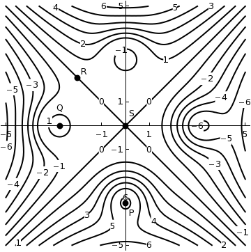
Each of the following functions has at most one critical point. Graph a few level curves and a few gradients and, on this basis alone, decide whether the critical point is a local maximum, a local minimum, a saddle point, or that there is no critical point.

For $f(x, y) = e^{-4 x^2 - 2 y^2}\text{,}$ type of critical point:

Local Maximum
Local Minimum
Saddle Point
No Critical Point

For $f(x, y) = e^{4 x^2 - 2 y^2}\text{,}$ type of critical point:

Local Maximum
Local Minimum
Saddle Point
No Critical Point

For $f(x, y) = 4 x^2+ 2 y^2+ 1\text{,}$ type of critical point:

Local Maximum
Local Minimum
Saddle Point
No Critical Point

For $f(x, y) = 4 x^2+ 2 y+ 1\text{,}$ type of critical point:

Local Maximum
Local Minimum
Saddle Point
No Critical Point

6.

Find the absolute minimum and absolute maximum of

\begin{equation*} f(x,y) = 19 - 10 x + 13 y \end{equation*}

on the closed triangular region with vertices $(0,0), (13, 0)$ and $(13, 17)\text{.}$

List the minimum/maximum values as well as the point(s) at which they occur. If a min or max occurs at multiple points separate the points with commas.

Minimum value:

Occurs at

Maximum value:

Occurs at

7.

Find the maximum and minimum values of $f(x, y) = xy$ on the ellipse $2\!x^{2} + y^{2} = 6\text{.}$

maximum value =

minimum value =

8.

Find $A$ and $B$ so that $f(x,y) = x^2 + Ay + y^2 + B$ has a local minimum at the point $(0, 2)\text{,}$ with $z$-coordinate 20.

$A =$

$B =$

9.

The contours of a function $f$ are shown in the figure below.

For each of the points shown, indicate whether you think it is a local maximum, local minimum, saddle point, or none of these.

(a) Point P is

a local maximum
a local minimum
a saddle point
none of these

(b) Point Q is

a local maximum
a local minimum
a saddle point
none of these

(c) Point R is

a local maximum
a local minimum
a saddle point
none of these

(d) Point S is

a local maximum
a local minimum
a saddle point
none of these

10.

Consider the three points $(2,3)\text{,}$ $(1,4)\text{,}$ and $(6,7)\text{.}$

(a) Supposed that at $(2,3)\text{,}$ we know that $f_x=f_y=0$ and $f_{xx} \lt 0\text{,}$ $f_{yy} > 0\text{,}$ and $f_{xy} = 0\text{.}$ What can we conclude about the behavior of this function near the point $(2,3)\text{?}$

(2,3) is a local maximum
(2,3) is a local minimum
(2,3) is a saddle point
(2,3) is a none of these

(b) Supposed that at $(1,4)\text{,}$ we know that $f_x=f_y=0$ and $f_{xx} \lt 0\text{,}$ $f_{yy} > 0\text{,}$ and $f_{xy} = 0\text{.}$ What can we conclude about the behavior of this function near the point $(1,4)\text{?}$

(1,4) is a local maximum
(1,4) is a local minimum
(1,4) is a saddle point
(1,4) is a none of these

(c) Supposed that at $(6,7)\text{,}$ we know that $f_x=f_y=0$ and $f_{xx} \lt 0\text{,}$ $f_{yy} = 0\text{,}$ and $f_{xy} \lt 0\text{.}$ What can we conclude about the behavior of this function near the point $(6,7)\text{?}$

(6,7) is a local maximum
(6,7) is a local minimum
(6,7) is a saddle point
(6,7) is a none of these

Using this information, on a separate sheet of paper sketch a possible contour diagram for $f\text{.}$

11.

Find three positive real numbers whose sum is 50 and whose product is a maximum.

Enter the three numbers separated by commas:

12.

A closed rectangular box has volume $44\,\mbox{cm}^3\text{.}$ What are the lengths of the edges giving the minimum surface area?

lengths =

(Give the three lengths as a comma separated list.)

13.

An open rectangular box has volume $50 \mbox{ cm}^3\text{.}$ What are the lengths of the edges giving the minimum surface area?

lengths =

(Give the three lengths as a comma separated list.)

14.

What is the shortest distance from the surface $x y + 15 x + z^2 = 201$ to the origin?

distance =

15.

Find the volume of the largest rectangular box with edges parallel to the axes that can be inscribed in the ellipsoid

\begin{equation*} \frac{x^2}{81} + \frac{y^2}{64} + \frac{z^2}{9} = 1 \end{equation*}

Hint: By symmetry, you can restrict your attention to the first octant (where $x, y, z \ge 0$), and assume your volume has the form $V = 8xyz\text{.}$ Then arguing by symmetry, you need only look for points which achieve the maximum which lie in the first octant.

Maximum volume:

16.

Design a rectangular milk carton box of width $w\text{,}$ length $l\text{,}$ and height $h$ which holds $454 \text{ cm}^3$ of milk. The sides of the box cost $2 \ \text{cents/cm}^2$ and the top and bottom cost $4\ \text{cents/cm}^2\text{.}$ Find the dimensions of the box that minimize the total cost of materials used.

width = , length = , height =

(Include units in your answers.) (Help with units.

/webwork2_files/helpFiles/Units.html

)

17.

Respond to each of the following prompts to solve the given optimization problem.

Let $f(x,y) = \sin(x)+\cos(y)\text{.}$ Determine the absolute maximum and minimum values of $f\text{.}$ At what points do these extreme values occur?
For a certain differentiable function $F$ of two variables $x$ and $y\text{,}$ its partial derivatives are

\begin{equation*} F_x(x,y) = x^2-y-4 \ \ \mbox{and} \ \ F_y(x,y) = -x + y - 2. \end{equation*}

Find each of the critical points of $F\text{,}$ and classify each as a local maximum, local minimum, or a saddle point.
Determine all critical points of $T(x,y) = 48 + 3xy - x^2y - xy^2$ and classify each as a local maximum, local minimum, or saddle point.
Find and classify all critical points of $g(x,y) = \frac{x^2}{2} + 3y^3 + 9y^2 - 3xy + 9y - 9x$
Find and classify all critical points of $z = f(x,y) = ye^{-x^2-2y^2}\text{.}$
Determine the absolute maximum and absolute minimum of $f(x,y) = 2 + 2x + 2y - x^2 - y^2$ on the triangular plate in the first quadrant bounded by the lines $x = 0\text{,}$ $y = 0\text{,}$ and $y = 9-x\text{.}$
Determine the absolute maximum and absolute minimum of $f(x,y) = 2 + 2x + 2y - x^2 - y^2$ over the closed disk of points $(x,y)$ such that $(x-1)^2 + (y-1)^2 \le 1\text{.}$
Find the point on the plane $z = 6 - 3x - 2y$ that lies closest to the origin.

18.

If a continuous function $f$ of a single variable has two critical numbers $c_1$ and $c_2$ at which $f$ has relative maximum values, then $f$ must have another critical number $c_3\text{,}$ because “it is impossible to have two mountains without some sort of valley in between. The other critical point can be a saddle point (a pass between the mountains) or a local minimum (a true valley).” (From Calculus in Vector Spaces by Lawrence J. Corwin and Robert H. Szczarb.) Consider the function $f$ defined by $f(x,y) = 4x^2e^y -2x^4 -e^{4y}\text{.}$ (From Ira Rosenholz in the Problems Section of the Mathematics Magazine, Vol. 60 NO. 1, February 1987.) Show that $f$ has exactly two critical points, and that $f$ has relative maximum values at each of these critical points. Explain how this function $f$ illustrates that it really is possible to have two mountains without some sort of valley in between. Use appropriate technology to draw the surface defined by $f$ to see graphically how this happens.

19.

If a continuous function $f$ of a single variable has exactly one critical number with a relative maximum at that critical point, then the value of $f$ at that critical point is an absolute maximum. In this exercise we see that the same is not always true for functions of two variables. Let $f(x,y) = 3xe^y-x^3-e^{3y}$ (from “The Only Critical Point in Town” Test by Ira Rosenholz and Lowell Smylie in the Mathematics Magazine, VOL 58 NO 3 May 1985.). Show that $f$ has exactly one critical point, has a relative maximum value at that critical point, but that $f$ has no absolute maximum value. Use appropriate technology to draw the surface defined by $f$ to see graphically how this happens.

20.

A manufacturer wants to procure rectangular boxes to ship its product. The boxes must contain 20 cubic feet of space. To be durable enough to ensure the safety of the product, the material for the sides of the boxes will cost $0.10 per square foot, while the material for the top and bottom will cost $0.25 per square foot. In this activity we will help the manufacturer determine the box of minimal cost.

What quantities are constant in this problem? What are the variables in this problem? Provide appropriate variable labels. What, if any, restrictions are there on the variables?
Using your variables from (a), determine a formula for the total cost $C$ of a box.
Your formula in part (b) might be in terms of three variables. If so, find a relationship between the variables, and then use this relationship to write $C$ as a function of only two independent variables.
Find the dimensions that minimize the cost of a box. Be sure to verify that you have a minimum cost.

21.

A rectangular box with length $x\text{,}$ width $y\text{,}$ and height $z$ is being built. The box is positioned so that one corner is stationed at the origin and the box lies in the first octant where $x\text{,}$ $y\text{,}$ and $z$ are all positive. There is an added constraint on how the box is constructed: it must fit underneath the plane with equation $x + 2y + 3z = 6\text{.}$ In fact, we will assume that the corner of the box “opposite” the origin must actually lie on this plane. The basic problem is to find the maximum volume of the box.

Sketch the plane $x + 2y + 3z = 6\text{,}$ as well as a picture of a potential box. Label everything appropriately.
Explain how you can use the fact that one corner of the box lies on the plane to write the volume of the box as a function of $x$ and $y$ only. Do so, and clearly show the formula you find for $V(x,y)\text{.}$
Find all critical points of $V\text{.}$ (Note that when finding the critical points, it is essential that you factor first to make the algebra easier.)
Without considering the current applied nature of the function $V\text{,}$ classify each critical point you found above as a local maximum, local minimum, or saddle point of $V\text{.}$
Determine the maximum volume of the box, justifying your answer completely with an appropriate discussion of the critical points of the function.
Now suppose that we instead stipulated that, while the vertex of the box opposite the origin still had to lie on the plane, we were only going to permit the sides of the box, $x$ and $y\text{,}$ to have values in a specified range (given below). That is, we now want to find the maximum value of $V$ on the closed, bounded region

\begin{equation*} \frac{1}{2} \le x \le 1, \ \ 1 \le y \le 2. \end{equation*}

Find the maximum volume of the box under this condition, justifying your answer fully.

22.

The airlines place restrictions on luggage that can be carried onto planes.

A carry-on bag can weigh no more than 40 lbs.
The length plus width plus height of a bag cannot exceed 45 inches.
The bag must fit in an overhead bin.

Let $x\text{,}$ $y\text{,}$ and $z$ be the length, width, and height (in inches) of a carry on bag. In this problem we find the dimensions of the bag of largest volume, $V = xyz\text{,}$ that satisfies the second restriction. Assume that we use all 45 inches to get a maximum volume. (Note that this bag of maximum volume might not satisfy the third restriction.)

Write the volume $V=V(x,y)$ as a function of just the two variables $x$ and $y\text{.}$
Explain why the domain over which $V$ is defined is the triangular region $R$ with vertices (0,0), (45,0), and (0,45).
Find the critical points, if any, of $V$ in the interior of the region $R\text{.}$
Find the maximum value of $V$ on the boundary of the region $R\text{,}$ and then determine the dimensions of a bag with maximum volume on the entire region $R\text{.}$ (Note that most carry-on bags sold today measure $22$ by $14$ by $9$ inches with a volume of $2772$ cubic inches, so that the bags will fit into the overhead bins.)

23.

According to The Song of Insects by G.W. Pierce (Harvard College Press, 1948) the sound of striped ground crickets chirping, in number of chirps per second, is related to the temperature. So the number of chirps per second could be a predictor of temperature. The data Pierce collected is shown in Table 2.6.11., where $x$ is the (average) number of chirps per second and $y$ is the temperature in degrees Fahrenheit.

A scatterplot of the data would show that, while the relationship between $x$ and $y$ is not exactly linear, it looks to have a linear pattern. It could be that the relationship is really linear but experimental error causes the data to be slightly inaccurate. Or perhaps the data is not linear, but only approximately linear.

Table 2.6.11. Crickets chirping.

$x$	$y$
$20.0$	$88.6$
$16.0$	$71.6$
$19.8$	$93.3$
$18.4$	$84.3$
$17.1$	$80.6$
$15.5$	$75.2$
$14.7$	$69.7$
$17.1$	$82.0$
$15.4$	$69.4$
$16.2$	$83.3$
$15.0$	$79.6$
$17.2$	$82.6$
$16.0$	$80.6$
$17.0$	$83.5$
$14.4$	$76.3$

If we want to use the data to make predications, then we need to fit a curve of some kind to the data. Since the cricket data appears roughly linear, we will fit a linear function $f$ of the form $f(x) = mx+b$ to the data. We will do this in such a way that we minimize the sums of the squares of the distances between the $y$ values of the data and the corresponding $y$ values of the line defined by $f\text{.}$ This type of fit is called a least squares approximation. If the data is represented by the points $(x_1,y_1)\text{,}$ $(x_2,y_2)\text{,}$ $\ldots\text{,}$ $(x_n,y_n)\text{,}$ then the square of the distance between $y_i$ and $f(x_i)$ is $(f(x_i)-y_i)^2 = (mx_i+b-y_i)^2\text{.}$ So our goal is to minimize the sum of these squares, of minimize the function $S$ defined by

\begin{equation*} S(m,b) = \sum_{i=1}^n (mx_i+b-y_i)^2. \end{equation*}

Calculate $S_m$ and $S_b\text{.}$
Solve the system $S_m(m,b) = 0$ and $S_b(m,b) = 0$ to show that the critical point satisfies

\begin{align*} m \amp = \frac{n\left(\sum_{i=1}^n x_iy_i\right) - \left(\sum_{i=1}^n x_i \right) \left(\sum_{i=1}^n y_i \right)}{n\left(\sum_{i=1}^n x_i^2 \right) - \left(\sum_{i=1}^n x_i \right)^2}\\ b \amp = \frac{\left(\sum_{i=1}^n y_i\right) \left(\sum_{i=1}^n x_i^2\right) - \left(\sum_{i=1}^n x_i \right) \left(\sum_{i=1}^n x_iy_i \right)}{n\left(\sum_{i=1}^n x_i^2 \right) - \left(\sum_{i=1}^n x_i \right)^2}. \end{align*}

(Hint: Don’t be daunted by these expressions, the system $S_m(m,b) = 0$ and $S_b(m,b) = 0$ is a system of two linear equations in the unknowns $m$ and $b\text{.}$ It might be easier to let $r=\sum_{i=1}^n x_i^2\text{,}$ $s=\sum_{i=1}^n x_i\text{,}$ $t = \sum_{i=1}^n y_i\text{,}$ and $u = \sum_{i=1}^n x_iy_i$ and write your equations using these constants.)
Use the Second Derivative Test to explain why the critical point gives a local minimum. Can you then explain why the critical point gives an absolute minimum?
Use the formula from part (b) to find the values of $m$ and $b$ that give the line of best fit in the least squares sense to the cricket data. Draw your line on the scatter plot to convince yourself that you have a well-fitting line.

Prev Top Next

\(x\)	\(y\)
\(20.0\)	\(88.6\)
\(16.0\)	\(71.6\)
\(19.8\)	\(93.3\)
\(18.4\)	\(84.3\)
\(17.1\)	\(80.6\)
\(15.5\)	\(75.2\)
\(14.7\)	\(69.7\)
\(17.1\)	\(82.0\)
\(15.4\)	\(69.4\)
\(16.2\)	\(83.3\)
\(15.0\)	\(79.6\)
\(17.2\)	\(82.6\)
\(16.0\)	\(80.6\)
\(17.0\)	\(83.5\)
\(14.4\)	\(76.3\)