Coordinated Multivariable Calculus

Subsection1.1.1Functions of Several Variables

Up to this point we have been concerned with functions of a single variable. What defined such a function is that every input in the domain produced a unique output in the range. We saw similar behavior in Preview Activity1.1.1, where each pair \((P,t)\) of inputs produces a unique output \(A(P,t)\text{.}\) Additionally, the two variables \(P\) and \(t\) had no real relation to each other. That is, we could choose any value of \(P\) without considering what value \(t\) might have, and we could select any value of \(t\) to use without regard to what value \(P\) might have. For that reason we say that the variables \(t\) and \(P\) are independent of each other. Thus, we call \(A = A(P,t)\) a function of the two independent variables \(P\) and \(t\text{.}\) This is the key idea in defining a function of two independent variables.

There is, of course, no reason to restrict ourselves to functions of only two variableswe can use any number of variables we like. For example,

defines \(f\) as a function of the three variables \(x\text{,}\) \(y\text{,}\) and \(z\text{.}\) In general, a function of \(n\) independent variables is a rule that assigns to an ordered \(n\)-tuple \((x_1, x_2, \ldots, x_n)\) in some set \(D\) exactly one real number.

Functions of two variables might model elevation on a map (the elevation at a point \((x,y)\) might be the value \(E(x,y)\)) or quantities like temperature or charge from physics.

As with functions of a single variable, it is important to understand the set of inputs for which the function is defined.

Subsection1.1.2Representing Functions of Two Variables

One of the techniques we use to study functions of one variable is to create a table of values. We can do the same for functions of two variables, except that our tables will have to allow us to keep track of both input variables. We can do this with a 2-dimensional table, where we list the \(x\)-values down the first column and the \(y\)-values across the first row. As an example, suppose we launch a projectile, using a golf club, a cannon, or some other device, from ground level. Under ideal conditions (ignoring wind resistance, spin, or any other forces except the force of gravity) the horizontal distance the object will travel depends on the initial velocity \(x\) the object is given, and the angle \(y\) at which it is launched. If we let \(f\) represent the horizontal distance the object travels, then \(f\) is a function of the two variables \(x\) and \(y\text{,}\) and we represent \(f\) in functional notation by

where \(g\) is the acceleration due to gravity. (Note that \(g\) is constant, 32 feet per second squared. We will derive this equation in a later section.) To create a table of values for \(f\text{,}\) we list the \(x\)-values down the first column and the \(y\)-values across the first row. The value \(f(x,y)\) is then displayed in the location where the \(x\) row intersects the \(y\) column, as shown in Table1.1.5 (where we measure \(x\) in feet per second and \(y\) in radians).

If \(f\) is a function of a single variable \(x\text{,}\) then we define the graph of \(f\) to be the set of points of the form \((x,f(x))\text{,}\) where \(x\) is in the domain of \(f\text{.}\) We then plot these points using the coordinate axes in order to visualize the graph. We can do a similar thing with functions of several variables. Table1.1.5 identifies points of the form \((x,y,f(x,y))\text{,}\) and we define the graph of \(f\) to be the set of these points.

We also often refer to the graph of a function \(f\) of two variables as the surface generated by \(f\text{.}\) Points in the form \((x,y,f(x,y))\) are in three dimensions, so plotting these points takes a bit more work than graphs of functions in two dimensions. To plot these three-dimensional points, we need to set up a coordinate system with three mutually perpendicular axes the \(x\)-axis, the \(y\)-axis, and the \(z\)-axis (called the coordinate axes). There are essentially two different ways we could set up a 3D coordinate system, as shown in Figure1.1.6; thus, before we can proceed, we need to establish a convention.

The distinction between these two figures is subtle, but important. In the coordinate system shown at left in Figure1.1.6, imagine that you are sitting on the positive \(z\)-axis next to the label \(z\text{.}\) Looking down at the \(x\)- and \(y\)-axes, you see that the \(y\)-axis is obtained by rotating the \(x\)-axis by 90\(^\circ\) in the clockwise direction. Again sitting on the positive \(z\)-axis in the coordinate system at right in Figure1.1.6, you see that the \(y\)-axis is obtained by rotating the \(x\)-axis by 90\(^\circ\) in the counterclockwise direction.

We call the coordinate system at right in Figure1.1.6 a right-hand system; if we point the index finger of our right hand along the positive \(x\)-axis and our middle finger along the positive \(y\)-axis, then our thumb points in the direction of the positive \(z\)-axis. Following mathematical conventions, we choose to use a right-hand system throughout this book.

Now that we have established a convention for a right-hand system, we can draw a graph of the distance function defined by \(f(x,y) = \frac{x^2 \sin(2y)}{g}\text{.}\) Note that the function \(f\) is continuous in both variables, so when we plot these points in the right hand coordinate system, we can connect them all to form a surface in 3-space. The graph of the distance function \(f\) is shown in Figure1.1.8.

There are many graphing tools available for drawing three-dimensional surfaces as indicated in the Preface (see Links to interactive graphics in Features of the Text). Since we will be able to visualize graphs of functions of two independent variables, but not functions of more than two variables, we will primarily deal with functions of two variables in this text. It is important to note, however, that the techniques we develop apply to functions of any number of variables.

Notation: We let \(\R^2\) denote the set of all ordered pairs of real numbers in the plane (two copies of the real number system) and let \(\R^3\) represent the set of all ordered triples of real numbers (which constitutes three-space).

Subsection1.1.3Some Standard Equations in Three-Space

In addition to graphing functions, we will also want to understand graphs of some simple equations in three dimensions. For example, in \(\R^2\text{,}\) the graphs of the equations \(x=a\) and \(y=b\text{,}\) where \(a\) and \(b\) are constants, are lines parallel to the coordinate axes. In the next activity we consider their three-dimensional analogues.

Activity1.1.5 shows that the equations where one independent variable is constant lead to planes parallel to ones that result from a pair of the coordinate axes. When we make the constant 0, we get the coordinate planes. The \(xy\)-plane satisfies \(z=0\text{,}\) the \(xz\)-plane satisfies \(y=0\text{,}\) and the \(yz\)-plane satisfies \(x=0\) (see Figure1.1.9).

On a related note, we define a circle in \(\R^2\) as the set of all points equidistant from a fixed point. In \(\R^3\text{,}\) we call the set of all points equidistant from a fixed point a sphere. To find the equation of a sphere, we need to understand how to calculate the distance between two points in three-space, and we explore this idea in the next activity.

Investigation1.1.6

Let \(P=(x_0, y_0, z_0)\) and \(Q=(x_1, y_1, z_1)\) be two points in \(\R^3\text{.}\) These two points form opposite vertices of a rectangular box whose sides are planes parallel to the coordinate planes as illustrated in Figure1.1.10, and the distance between \(P\) and \(Q\) is the length of the blue diagonal shown in Figure1.1.10.

Answer

1. \(S = (x_1,y_0,z_0)\) and \(R = (x_1,y_1,z_0)\) are the two points that aren't given. The legs of the right triangle are \(PS\text{,}\) which has length \(x_1 - x_0\text{,}\) and \(SR\text{,}\) which has length \(y_1 - y_0\text{.}\) The hypotenuse \(PR\) therefore has length \(\sqrt{(x_1-x_0)^2 + (y_1 - y_0)^2}\text{.}\)

2. Applying the Pythagorean Theorem to the triangle \(PRQ\) gives \(PR^2 + QR^2 = PQ^2\text{.}\) Noting that \(QR\) has length \(z_1 - z_0\text{,}\) we can plug in \(\sqrt{(x_1-x_0)^2 + (y_1 - y_0)^2}\) for \(PR\) (found in the previous part) to solve for \(PQ\) and obvain the formula given.

The formula developed in Investigation1.1.6 is important to remember.

Equation (1.1.1) can be used to derive the formula for a sphere centered at a point \((x_0,y_0,z_0)\) with radius \(r\text{.}\) Since the distance from any point \((x,y,z)\) on such a sphere to the point \((x_0,y_0,z_0)\) is \(r\text{,}\) the point \((x,y,z)\) will satisfy the equation

Squaring both sides, we come to the standard equation for a sphere.

This makes sense if we compare this equation to its two-dimensional analogue, the equation of a circle of radius \(r\) in the plane centered at \((x_0,y_0)\text{:}\)

Subsection1.1.4Traces

When we study functions of several variables we are often interested in how each individual variable affects the function in and of itself. In Preview Activity1.1.1, we saw that the amount of money in an account depends on the amount initially invested and the duration of the investment. However, if we fix the initial investment, the amount of money in the account depends only on the duration of the investment, and if we set the duration of the investment constant, then the amount of money in the account depends only on the initial investment. This idea of keeping one variable constant while we allow the other to change will be an important tool for us when studying functions of several variables.

As another example, consider again the distance function \(f\) defined by

where \(x\) is the initial velocity of an object in feet per second, \(y\) is the launch angle in radians, and \(g\) is the acceleration due to gravity (32 feet per second squared). If we hold the launch angle constant at \(y=0.6\) radians, we can consider \(f\) a function of the initial velocity alone. In this case we have

We can plot this curve on the surface by tracing out the points on the surface when \(y = 0.6\text{,}\) as shown at left in Figure1.1.14. The formula clearly shows that \(f\) is quadratic in the \(x\)-direction. More descriptively, as we increase the launch velocity while keeping the launch angle constant, the horizontal distance the object travels increases proportional to the square of the initial velocity.

Similarly, if we fix the initial velocity at 150 feet per second, we can consider the distance as a function of the launch angle only. In this case we have

We can again plot this curve on the surface by tracing out the points on the surface when \(x=150\text{,}\) as shown at right in Figure1.1.14. The formula clearly show that \(f\) is sinusoidal in the \(y\)-direction. More descriptively, as we increase the launch angle while keeping the initial velocity constant, the horizontal distance traveled by the object is proportional to the sine of twice the launch angle.

The curves we define when we fix one of the independent variables in our two variable function are called traces.

Understanding trends in the behavior of functions of two variables can be challenging, as can sketching their graphs; traces help us with each of these tasks.

Example1.1.16

Which of the following graphs depicts which function, and why?

\begin{align*} f(x,y) \amp = x^2 + y^2 \\ g(x,y) \amp = \sqrt{x^2 + y^2} \end{align*}

Hint

Look at the traces. For a fixed \(y\)-value \(c\text{,}\) we see that the \(y\)-trace of \(f\) is given by \(y = f(x,c) = x^2 + c^2\text{,}\) an equation for a parabola with vertex \((0,c^2)\text{.}\) So, for example, \(c = 0\) gives the parabola \(y = x^2\text{.}\)

On the other hand, the \(y\)-trace of \(g\) at \(y = 0\) is described by the equation \(y = g(x,0) = \sqrt{x^2 + 0^2} = \sqrt{x^2} = |x|\text{.}\)

Subsection1.1.5Contour Maps and Level Curves

We have all seen topographic maps such as the one of the Porcupine Mountains in the upper peninsula of Michigan shown in Figure1.1.18.¹Map source: Michigan Department of Natural Resources, with permission of the Michigan DNR and Bob Wild. The curves on these maps show the regions of constant altitude. The contours also depict changes in altitude: contours that are close together signify steep ascents or descents, while contours that are far apart indicate only slight changes in elevation. Thus, contour maps tell us a lot about three-dimensional surfaces. Mathematically, if \(f(x,y)\) represents the altitude at the point \((x,y)\text{,}\) then each contour is the graph of an equation of the form \(f(x,y) = k\text{,}\) for some constant \(k\text{.}\)

Curves on a surface that describe points at the same height or level are called level curves.

Topographical maps can be used to create a three-dimensional surface from the two-dimensional contours or level curves. For example, level curves of the distance function defined by \(f(x,y) = \frac{x^2 \sin(2y)}{32}\) plotted in the \(xy\)-plane are shown at left in Figure1.1.20. If we lift these contours and plot them at their respective heights, then we get a picture of the surface itself, as illustrated at right in Figure1.1.20.

The use of level curves and traces can help us construct the graph of a function of two variables.

Activity1.1.9

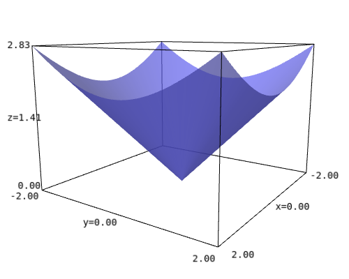
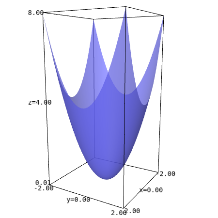
1. Let \(f(x,y) = x^2+y^2\text{.}\) Draw the level curves \(f(x,y) = k\) for \(k=1\text{,}\) \(k=2\text{,}\) \(k=3\text{,}\) and \(k=4\) on the left set of axes given in Figure1.1.21. (You decide on the scale of the axes.) Explain what the surface defined by \(f\) looks like.

2. Let \(g(x,y) = \sqrt{x^2+y^2}\text{.}\) Draw the level curves \(g(x,y) = k\) for \(k=1\text{,}\) \(k=2\text{,}\) \(k=3\text{,}\) and \(k=4\) on the right set of axes given in Figure1.1.21. (You decide on the scale of the axes.) Explain what the surface defined by \(g\) looks like.

3. Compare and contrast the graphs of \(f\) and \(g\text{.}\) How are they alike? How are they different? Use traces for each function to help answer these questions.

The traces and level curves of a function of two variables are curves in space. In order to understand these traces and level curves better, we will first spend some time learning about vectors and vector-valued functions in the next few sections and return to our study of functions of several variables once we have those more mathematical tools to support their study.

Subsection1.1.6A gallery of functions

We end this section by considering a collection of functions and illustrating their graphs and some level curves.

Subsection1.1.7Summary

• A function \(f\) of several variables is a rule that assigns a unique number to an ordered collection of independent inputs. The domain of a function of several variables is the set of all inputs for which the function is defined.

• In \(\R^3\text{,}\) the distance between points \(P=(x_0, y_0, z_0)\) and \(Q=(x_1, y_1, z_1)\) (denoted as \(|PQ|\)) is given by the formula

  \begin{equation*} |PQ| = \sqrt{(x_1-x_0)^2 + (y_1-y_0)^2 + (z_1-z_0)^2}. \end{equation*}

  and thus the equation of a sphere with center \((x_0,y_0,z_0)\) and radius \(r\) is

  \begin{equation*} (x-x_0)^2 + (y-y_0)^2 + (z-z_0)^2 = r^2. \end{equation*}

• A trace of a function \(f\) of two independent variables \(x\) and \(y\) is a curve of the form \(z = f(c,y)\) or \(z = f(x,c)\text{,}\) where \(c\) is a constant. A trace tells us how the function depends on a single independent variable if we treat the other independent variable as a constant.

• A level curve of a function \(f\) of two independent variables \(x\) and \(y\) is a curve of the form \(k = f(x,y)\text{,}\) where \(k\) is a constant. A level curve describes the set of inputs that lead to a specific output of the function.