CC Second Derivative Test

Section 4.2 Second Derivative Test

Motivating Questions

What is concavity and how we determine the concavity of a function?
How can the second derivative of a function be used to help identify extreme values of the function?
What are inflection points, and what do they tell us about the graph of a function?

This section corresponds to 3.3 Concavity, 3.4 Second Derivative Test, and 3.5 Curve Sketching in the workbook.

We have seen how the first derivative of a function can help us determine when a function is increasing or decreasing. We have also seen how we can use that information to determine when a function reaches a maximum or minimum point. We will now explore what the second derivative of a function tells us.

🔗

Subsection 4.2.1 Concavity

🔗

In addition to asking whether a function is increasing or decreasing, it is also natural to inquire how a function is increasing or decreasing. There are three basic behaviors that an increasing function can demonstrate on an interval, as pictured below in Figure 4.2.1: the function can increase more and more rapidly, it can increase at the same rate, or it can increase in a way that is slowing down. Fundamentally, we are beginning to think about how a particular curve bends, with the natural comparison being made to lines, which don’t bend at all. More than this, we want to understand how the bend in a function’s graph is tied to behavior characterized by the first derivative of the function.

🔗
Figure 4.2.1. Three functions that are all increasing, but doing so at an increasing rate, at a constant rate, and at a decreasing rate, respectively.

🔗

On the leftmost curve in Figure 4.2.1, draw a sequence of tangent lines to the curve. As we move from left to right, the slopes of those tangent lines will increase. Therefore, the rate of change of the pictured function is increasing, and this explains why we say this function is increasing at an increasing rate. For the rightmost graph in Figure 4.2.1, observe that as

x

increases, the function increases, but the slopes of the tangent lines decrease. This function is increasing at a decreasing rate.

🔗

Similar options hold for how a function can decrease. Here we must be extra careful with our language, because decreasing functions involve negative slopes.

Negative numbers present an interesting tension between common language and mathematical language. For example, it can be tempting to say that “

- 100

is bigger than

- 2 .

” But we must remember that “greater than” describes how numbers lie on a number line:

x > y

provided that

x

lies to the right of

y .

So of course,

- 100

is less than

- 2 .

Informally, it might be helpful to say that “

- 100

is more negative than

- 2 .

”

🔗
Figure 4.2.2. From left to right, three functions that are all decreasing, but doing so in different ways.

🔗

Now consider the three graphs shown above in Figure 4.2.2. The middle graph depicts a function decreasing at a constant rate. Now draw a sequence of tangent lines on the first curve. We see that the slopes of these lines get closer to zero — meaning they get less and less negative — as we move from left to right. That means that the values of the first derivative, while all negative, are increasing, and thus we say that the leftmost curve is decreasing at an increasing rate.

🔗

This leaves only the rightmost curve in Figure 4.2.2 to consider. For that function, the slopes of the tangent lines are negative throughout the pictured interval, but as we move from left to right, the slopes get more and more negative as they get steeper. Hence the slope of the curve is decreasing, and we say that the function is decreasing at a decreasing rate.

🔗

We now introduce the notion of concavity, which provides simpler language to describe these behaviors. When a curve opens upward on a given interval, like the parabola

y = x^{2}

or the exponential growth function

y = e^{x},

we say that the curve is concave up on that interval. Likewise, when a curve opens down, like the parabola

y = - x^{2}

or the negative exponential function

y = - e^{x},

we say that the function is concave down. Concavity is linked to both the first and second derivatives of the function.

🔗

In Figure 4.2.3 below, we see two functions and a sequence of tangent lines to each. The lefthand plot shows a function that is concave up; observe that here the tangent lines always lie below the curve itself, and the slopes of the tangent lines are increasing as we move from left to right. In other words, the graph of

y = f (x)

is concave up on the interval shown because its derivative,

f^{'},

is increasing on that interval. Similarly, the righthand plot in Figure 4.2.3 depicts a function that is concave down; in this case, we see that the tangent lines always lie above the curve and that the slopes of the tangent lines are decreasing as we move from left to right. The fact that its derivative,

f^{'},

is decreasing makes

f

concave down on the interval shown.

🔗
Figure 4.2.3. At left, a function that is concave up; at right, one that is concave down.

🔗

We state these most recent observations formally as the definitions of the terms concave up and concave down.

🔗

Concavity.

🔗

Let

f

be a differentiable function on an interval

(a, b) .

Then

f

is concave up on

(a, b)

if and only if

f^{″} > 0,

that is

f^{'}

is increasing, on

(a, b);

f

is concave down on

(a, b)

if and only if

f^{″} < 0,

that is

f^{'}

is decreasing, on

(a, b) .

🔗

Exploring the context of position, velocity, and acceleration is an excellent way to understand how a function, its first derivative, and its second derivative are related to one another.

Example 4.2.4.

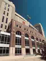
The position of a car driving along a straight road at time

t

in minutes is given by the function

y = s (t)

that is pictured below in Figure 4.2.5. The car’s position function has units measured in thousands of feet.

Figure 4.2.5. The graph of $y = s (t),$ the position of the car (measured in thousands of feet from its starting location) at time $t$ in minutes.

On what intervals is the position function $y = s (t)$ increasing? Decreasing? Why?
On which intervals is the velocity function $y = v (t) = s^{'} (t)$ increasing? Decreasing? Neither? Why?
Acceleration is defined to be the instantaneous rate of change of velocity, as the acceleration of an object measures the rate at which the velocity of the object is changing. Say that the car’s acceleration function is named $a (t) .$ How is $a (t)$ computed from $v (t) ?$ How is $a (t)$ computed from $s (t) ?$ Explain.
What can you say about $s^{″}$ whenever $s^{'}$ is increasing? Why?
Using only the words increasing, decreasing, constant, concave up, concave down, and linear, complete the following sentences. For the position function $s$ with velocity $v$ and acceleration $a,$
- on an interval where $v$ is positive, $s$ is .
- on an interval where $v$ is negative, $s$ is .
- on an interval where $v$ is zero, $s$ is .
- on an interval where $a$ is positive, $v$ is .
- on an interval where $a$ is negative, $v$ is .
- on an interval where $a$ is zero, $v$ is .
- on an interval where $a$ is positive, $s$ is .
- on an interval where $a$ is negative, $s$ is .
- on an interval where $a$ is zero, $s$ is .

Hint.

Remember that a function is increasing on an interval if and only if its first derivative is positive on the interval.
See (a).
Remember that the first derivative of a function measures its instantaneous rate of change.
Think about how $s^{″} (t) = [s^{'} (t)]^{'} .$
Be very careful with your letters: $s,$ $v,$ and $a .$

Answer.

Increasing: $0 < t < 2,$ $3 < t < 5,$ $6 < t < 8,$ and $9 < t < 11 .$ Decreasing: never.
Velocity is increasing on $0 < t < 1.1,$ $3 < t < 4.1,$ $6 < t < 7.1,$ and $9 < t < 10.1;$ $y = v (t)$ is decreasing on $1.1 < t < 2,$ $4.1 < t < 5,$ $7.1 < t < 8,$ and $10.1 < t < 11 .$ Velocity is neither increasing nor decreasing (i.e. the velocity is constant) on $2 < t < 3,$ $5 < t < 6,$ $8 < t < 9,$ and $11 < t < 12 .$
$a (t) = v^{'} (t)$ and $a (t) = s^{″} (t) .$
$s^{″} (t)$ is positive since $s^{'} (t)$ is increasing.
- increasing.
- decreasing.
- constant.
- increasing.
- decreasing.
- constant.
- concave up.
- concave down.
- linear.

Solution.

The position function $y = s (t)$ is increasing on the intervals $0 < t < 2,$ $3 < t < 5,$ $6 < t < 8,$ and $9 < t < 11$ because $s^{'} (t)$ is positive at every point in such intervals. Furthermore, $s (t)$ is never decreasing because its derivative is never negative.
The velocity function $y = v (t)$ appears to be increasing on the intervals $0 < t < 1.1,$ $3 < t < 4.1,$ $6 < t < 7.1,$ and $9 < t < 10.1 .$ This is because the curve $y = s (t)$ is concave up on these intervals, which corresponds to an increasing first derivative $y = s^{'} (t) .$ Similarly, $y = v (t)$ appears to be decreasing on the intervals $1.1 < t < 2,$ $4.1 < t < 5,$ $7.1 < t < 8,$ and $10.1 < t < 11 .$ This is due to the curve $y = s (t)$ being concave down on these intervals, corresponding to a decreasing first derivative $y = s^{'} (t) .$ On the intervals $2 < t < 3,$ $5 < t < 6,$ $8 < t < 9,$ and $11 < t < 12,$ the curve $y = s (t)$ is constant, and thus linear, so $s$ is neither concave up nor concave down. On these intervals, then, the velocity function is constant.
Since $a (t)$ is the instantaneous rate of change of $v (t),$ we can say $a (t) = v^{'} (t) .$ Moreover, because $v (t) = s^{'} (t),$ it follows that $a (t) = v^{'} (t) = [s^{'} (t)]^{'} = s^{″} (t),$ so acceleration is the second derivative of position.
Since $s^{″} (t)$ is the first derivative of $s^{'} (t),$ then whenever $s^{'} (t)$ is increasing, $s^{″} (t)$ must be positive.
For the position function $s (t)$ with velocity $v (t)$ and acceleration $a (t),$
- on an interval where $v (t)$ is positive, $s (t)$ is increasing.
- on an interval where $v (t)$ is negative, $s (t)$ is decreasing.
- on an interval where $v (t)$ is zero, $s (t)$ is constant.
- on an interval where $a (t)$ is positive, $v (t)$ is increasing.
- on an interval where $a (t)$ is negative, $v (t)$ is decreasing.
- on an interval where $a (t)$ is zero, $v (t)$ is constant.
- on an interval where $a (t)$ is positive, $s (t)$ is concave up.
- on an interval where $a (t)$ is negative, $s (t)$ is concave down.
- on an interval where $a (t)$ is zero, $s (t)$ is linear.

🔗

Subsection 4.2.2 The Second Derivative Test

🔗

Recall that the second derivative of a function tells us several important things about the behavior of the function itself. For instance, if

f^{″}

is positive on an interval, then

f^{'}

is increasing on that interval and

f

is concave up on that interval. This also tells us that throughout that interval the tangent line to

y = f (x)

lies below the curve at every point. As seen in Figure 4.2.6 below, at a point where

f^{'} (c) = 0,

the sign of the second derivative determines whether

f

has a local minimum or local maximum at the critical number

x = c .

🔗
Figure 4.2.6. Four possible graphs of a function $f$ with a horizontal tangent line at a critical point.

🔗

In Figure 4.2.6 above, we see the four possibilities for a function

f

that has a critical number

c

at which

f^{'} (c) = 0,

provided we can find an interval around

c

on which

f^{″} (c)

is not zero, except possibly at

p .

On either side of the critical number,

f^{″}

can be either positive or negative, and hence

f

can be either concave up or concave down. In the first two graphs,

f

does not change concavity at

c

and

f

has either a local minimum or local maximum in those situations. In particular, if

f^{'} (c) = 0

and

f^{″} (c) < 0,

then

f

is concave down at

c

with a horizontal tangent line, so

f

has a local maximum there. This fact, along with the corresponding statement for when

f^{″} (c)

is positive, is the substance of the second derivative test.

🔗

Second Derivative Test.

🔗

c

is a critical number of a continuous function

f

such that

f^{'} (c) = 0

and

f^{″} (c) \neq 0,

then

f

has a relative maximum at

c

if and only if

f^{″} (c) < 0,

and

f

has a relative minimum at

c

if and only if

f^{″} (c) > 0 .

🔗

In the event that

f^{″} (c) = 0,

the second derivative test is inconclusive. That is, the test doesn’t provide us any information. This is because if

f^{″} (c) = 0,

it is possible that

f

has a local minimum, local maximum, or neither.

Consider the functions

f (x) = x^{4},

g (x) = - x^{4},

and

h (x) = x^{3}

at the critical point

x = 0 .

🔗

Just as a first derivative sign chart reveals all of the increasing and decreasing behavior of a function, we can construct a second derivative sign chart that demonstrates all of the important information involving concavity.

Example 4.2.7.

Let

f

be a function whose first derivative is

f^{'} (x) = 3 x^{4} - 9 x^{2} .

Construct both first and second derivative sign charts for

f;

fully discuss where

f

is increasing, decreasing, concave up, and concave down; identify all relative extreme values; and sketch a possible graph of

f .

Solution.

Since we know

f^{'} (x) = 3 x^{4} - 9 x^{2},

we can find the critical numbers of

f

by solving

3 x^{4} - 9 x^{2} = 0

(since

f^{'}

exists everywhere, then there are no critical numbers for which

f^{'} (x) = D N E .

Factoring, we observe that

0 = 3 x^{2} (x^{2} - 3) = 3 x^{2} (x + \sqrt{3}) (x - \sqrt{3}),

so that

x = 0, \pm \sqrt{3}

are the three critical numbers of

f .

The first derivative sign chart for

f

is given below in Figure 4.2.8.

Figure 4.2.8. The first derivative sign chart for $f$ when $f^{'} (x) = 3 x^{4} - 9 x^{2} = 3 x^{2} (x^{2} - 3) .$

We see that

f

is increasing on the intervals

(- \infty, - \sqrt{3})

and

(\sqrt{3}, \infty),

and

f

is decreasing on

(- \sqrt{3}, 0)

and

(0, \sqrt{3}) .

By the first derivative test, this information tells us that

f

has a local maximum at

x = - \sqrt{3}

and a local minimum at

x = \sqrt{3} .

Although

f

also has a critical number at

x = 0,

neither a maximum nor minimum occurs there since

f^{'}

does not change sign at

x = 0 .

Next, we move on to investigate concavity. Differentiating

f^{'} (x) = 3 x^{4} - 9 x^{2},

we see that

f^{″} (x) = 12 x^{3} - 18 x .

Since we are interested in knowing the intervals on which

f^{″}

is positive and negative, we first find where

f^{″} (x) = 0 .

Observe that

0 = 12 x^{3} - 18 x = 12 x (x^{2} - \frac{3}{2}) = 12 x (x + \sqrt{\frac{3}{2}}) (x - \sqrt{\frac{3}{2}}) .

This equation has solutions

x = 0, \pm \sqrt{\frac{3}{2}} .

Building a sign chart for

f^{″}

in the exact same way we do for

f^{'},

we see the result shown below in Figure 4.2.9.

Figure 4.2.9. The second derivative sign chart for $f$ when $f^{″} (x) = 12 x^{3} - 18 x = 12 x^{2} (x^{2} - \sqrt{\frac{3}{2}}) .$

Therefore

f

is concave down on the intervals

(- \infty, - \sqrt{\frac{3}{2}})

and

(0, \sqrt{\frac{3}{2}}),

and concave up on

(- \sqrt{\frac{3}{2}}, 0)

and

(\sqrt{\frac{3}{2}}, \infty) .

Putting all of this information together, we now see a complete and accurate possible graph of

f

in Figure 4.2.10.

Figure 4.2.10. A possible graph of the function $f$ in Example 4.2.7.

The point

A = (- \sqrt{3}, f (- \sqrt{3}))

is a local maximum, because

f

is increasing prior to

A

and decreasing after; similarly, the point

E = (\sqrt{3}, f (\sqrt{3})

is a local minimum. Note, too, that

f

is concave down at

A

and concave up at

E,

which is consistent both with our second derivative sign chart and the second derivative test. At points

B

and

D,

concavity changes, as we saw in the results of the second derivative sign chart in Figure 4.2.9. Finally, at point

C,

f

has a critical point with a horizontal tangent line, but neither a maximum nor a minimum occurs there, since

f

is decreasing both before and after

C .

It is also the case that concavity changes at

C .

While we completely understand where

f

is increasing and decreasing, where

f

is concave up and concave down, and where

f

has relative extrema, we do not know any specific information about the

y

-coordinates of points on the curve. For instance, while we know that

f

has a local maximum at

x = - \sqrt{3},

we don’t know the value of that maximum because we do not know

f (- \sqrt{3}) .

Any vertical translation of our sketch of

f

in Figure 4.2.10 would satisfy the given criteria for

f .

🔗

Points

B,

C,

and

D

in Figure 4.2.10 are locations at which the concavity of

f

changes. We give a special name to any such point.

🔗

Inflection Point.

🔗

Let

f

be a continuous function. If

p

is a point in the domain of

f

at which

f

changes concavity, then we say that

(p, f (p))

is an inflection point (or point of inflection) of

f .

🔗

Just as we look for locations where

f

changes from increasing to decreasing by considering the behavior at points

x = c

where

f^{'} (c) = 0

f^{'} (c)

is undefined, so too we find points

x = p

where

f^{″} (p) = 0

f^{″} (p)

is undefined to see if there are points of inflection at these locations.

🔗

At this point in our study, it is important to remind ourselves of the big picture that derivatives help to paint: the sign of the first derivative

f^{'}

tells us whether the function

f

is increasing or decreasing, while the sign of the second derivative

f^{″}

tells us how the function

f

is increasing or decreasing.

Example 4.2.11.

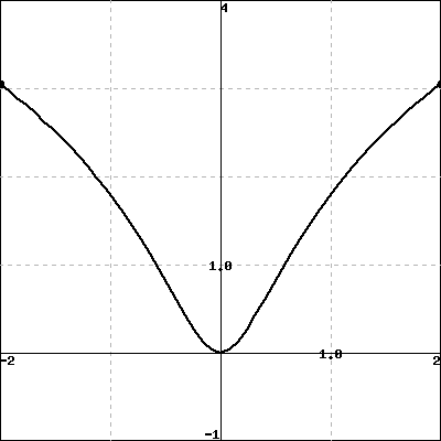
Suppose that

g

is a function whose second derivative,

g^{″},

is given by the graph in Figure 4.2.12 below.

Figure 4.2.12. The graph of $y = g^{″} (x) .$

Find the $x$ -coordinates of all points of inflection of $g .$
Fully describe the concavity of $g$ by making an appropriate sign chart.
Suppose you are given that $g^{'} (- 1.67857351) = 0 .$ Is there a local maximum, local minimum, or neither (for the function $g$ ) at this critical number of $g,$ or is it impossible to say? Why?
Assuming that $g^{″} (x)$ is a polynomial (and that all important behavior of $g^{″}$ is seen in the graph above), what degree polynomial do you think $g (x)$ is? Why?

Hint.

What must be true of $g^{″} (x)$ at a point of inflection?
Use the given graph to decide where $g^{″}$ is positive and negative.
What does the second derivative test say?
Can you guess a formula for $g^{″} (x)$ based on its graph?

Answer.

$x = - 1$ is an inflection point of $g .$
$g$ is concave up for $x < - 1$ and concave down for $x > - 1 .$
$g$ has a local minimum at $x = - 1.67857351 .$
$g$ is a degree 5 polynomial.

Solution.

Based on the given graph of $g^{″},$ the only point at which $g^{″}$ changes sign is $x = - 1,$ so this is the only inflection point of $g .$
Note that $g^{″} (x) > 0$ for $x < - 1$ and $g^{″} (x) < 0$ for $x > - 1 .$ This tells us that $g$ is concave up for $x < - 1$ and concave down for $x > - 1 .$
Given that $g^{'} (- 1.67857351) = 0,$ we know that $x = - 1.68757351$ is a critical number for $g .$ Additionally, the graph of $y = g^{″} (x)$ shows that $g^{″} (- 1.67857351) > 0,$ so we infer that $g$ is concave up at $x$ -values near $- 1.67857351 .$ The second derivative test allows us to conclude that $g$ has a local minimum at $x = - 1.67857351 .$
As seen in the given graph, since $g^{″}$ has a zero of multiplicity 1 at $x = - 1$ and a zero of multiplicity 2 at $x = 2,$ it appears that $g^{″}$ is a degree 3 polynomial. If so, then $g^{'}$ is a degree 4 polynomial, and $g$ is a degree 5 polynomial.

🔗

As we will see in more detail in the following section, derivatives also help us to understand families of functions that differ only by changing one or more parameters. For instance, we might be interested in understanding the behavior of all functions of the form

f (x) = a (x - h)^{2} + k

where

a,

h,

and

k

are parameters. Each parameter has considerable impact on how the graph appears.

🔗

Subsection 4.2.3 Summary

🔗

The Second Derivative Test tells us that given a twice differentiable function $f,$ if $f^{'} (c) = 0$ and $f^{″} (c) \neq 0,$ the sign of $f^{″}$ tells us the concavity of $f$ and hence whether $f$ has a maximum or minimum at $x = c .$ In particular, if $f^{'} (c) = 0$ and $f^{″} (c) < 0,$ then $f$ is concave down at $x = c$ and $f$ has a local maximum there, while if $f^{'} (c) = 0$ and $f^{″} (c) > 0,$ then $f$ has a local minimum at $x = c .$
The Second Derivative Test can be used only if $f$ is twice differentiable and $f^{″} (c) \neq 0$ at the critical number $x = c .$ If both $f^{'} (c) = 0$ and $f^{″} (c) = 0,$ then the second derivative test does not tell us whether $f$ has a local extremum at $x = c$ or not.

🔗

Exercises 4.2.4 Exercises

🔗

1. Concavity and inflection points.

🔗

PTX:ERROR: WeBWorK problem UNL-Problems/104-Problems/concavity6.pg with seed 111 does not return valid XML It may not be PTX compatible Use -a to halt with returned content

🔗

2. Finding critical points and inflection points.

🔗

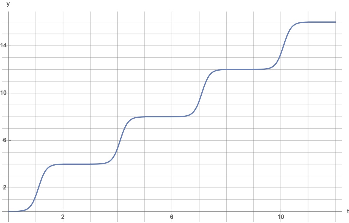
Use a graph below of

f (x) = \ln (5 x^{2} + 1)

to estimate the

x

-values of any critical points and inflection points of

f (x) .

🔗

critical points (enter as a comma-separated list):

x =

🔗

inflection points (enter as a comma-separated list):

x =

🔗

Next, use derivatives to find the

x

-values of any critical points and inflection points exactly.

🔗

critical points (enter as a comma-separated list):

x =

🔗

inflection points (enter as a comma-separated list):

x =

🔗

3. Finding inflection points.

🔗

Find the inflection points of

f (x) = 8 x^{4} + 110 x^{3} - 42 x^{2} + 14 .

(Give your answers as a comma separated list, e.g., 3,-2.)

🔗

inflection points =

🔗

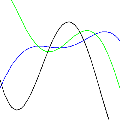
4. Matching graphs of $f, f^{'}, f^{″}$ .

🔗

The following shows graphs of three functions, A (in black), B (in blue), and C (in green). If these are the graphs of three functions

f,

f^{'},

and

f^{″},

identify which is which.

🔗

(Click on the graph to get a larger version.)

🔗

(For each enter A, B or C).

🔗

f =

;

f^{'} =

;

f^{″} =

🔗

5. Second derivative test.

🔗

PTX:ERROR: WeBWorK problem UNL-Problems/104-Problems/second_der_test1.pg with seed 115 does not return valid XML It may not be PTX compatible Use -a to halt with returned content

🔗

6. Curve sketching computations.

🔗

PTX:ERROR: WeBWorK problem UNL-Problems/104-Problems/second_der_test7.pg with seed 116 does not have a statement tag Maybe it uses something other than BEGIN_TEXT or BEGIN_PGML to print the statement in its PG code Use -a to halt with returned content

🔗

7. Using a derivative graph to analyze a function.

🔗

This problem concerns a function about which the following information is known:

$f$ is a differentiable function defined at every real number $x$
$f (0) = - \frac{1}{2}$
$y = f^{'} (x)$ has its graph given at center in Figure 4.2.13

Figure 4.2.13. At center, a graph of $y = f^{'} (x);$ at left, axes for plotting $y = f (x);$ at right, axes for plotting $y = f^{″} (x) .$

🔗

Construct a first derivative sign chart for $f .$ Clearly identify all critical numbers of $f,$ where $f$ is increasing and decreasing, and where $f$ has local extrema.
On the right-hand axes, sketch an approximate graph of $y = f^{″} (x) .$
Construct a second derivative sign chart for $f .$ Clearly identify where $f$ is concave up and concave down, as well as all inflection points.
On the left-hand axes, sketch a possible graph of $y = f (x) .$

🔗

8. Using derivative tests.

🔗

Suppose that

g

is a differentiable function and

g^{'} (2) = 0 .

In addition, suppose that on

1 < x < 2

and

2 < x < 3

it is known that

g^{'} (x)

is positive.

Does $g$ have a local maximum, local minimum, or neither at $x = 2 ?$ Why?
Suppose that $g^{″} (x)$ exists for every $x$ such that $1 < x < 3 .$ Reasoning graphically, describe the behavior of $g^{″} (x)$ for $x$ -values near $2 .$
Besides being a critical number of $g,$ what is special about the value $x = 2$ in terms of the behavior of the graph of $g ?$

🔗

9. Using a derivative graph to analyze a function.

🔗

Suppose that

h

is a differentiable function whose first derivative is given by the graph in Figure 4.2.14.

🔗

How many real number solutions can the equation $h (x) = 0$ have? Why?
If $h (x) = 0$ has two distinct real solutions, what can you say about the signs of the two solutions? Why?
Assume that $lim_{x \to \infty} h^{'} (x) = 3,$ as appears to be indicated in Figure 4.2.14. How will the graph of $y = h (x)$ appear as $x \to \infty ?$ Why?
Describe the concavity of $y = h (x)$ as fully as you can from the provided information.

Figure 4.2.14. The graph of $y = h^{'} (x) .$

🔗

10. Applying derivative tests.

🔗

Let

p

be a function whose second derivative is

p^{″} (x) = (x + 1) (x - 2) e^{- x} .

Construct a second derivative sign chart for $p$ and determine all inflection points of $p .$
Suppose you also know that $x = (\sqrt{5} - 1) / 2$ is a critical number of $p .$ Does $p$ have a local minimum, local maximum, or neither at $x = (\sqrt{5} - 1) / 2 ?$ Why?
If the point $(2, \frac{12}{e^{2}})$ lies on the graph of $y = p (x)$ and $p^{'} (2) = - \frac{5}{e^{2}},$ find the equation of the tangent line to $y = p (x)$ at the point where $x = 2 .$ Does the tangent line lie above the curve, below the curve, or neither at this value? Why?

Prev Top Next

Section 4.2 Second Derivative Test

Motivating Questions

Subsection 4.2.1 Concavity

Concavity.

Example 4.2.4.

Subsection 4.2.2 The Second Derivative Test

Second Derivative Test.

Example 4.2.7.

Inflection Point.

Example 4.2.11.

Subsection 4.2.3 Summary

Exercises 4.2.4 Exercises

1. Concavity and inflection points.

2. Finding critical points and inflection points.

3. Finding inflection points.

4. Matching graphs of f,f′,f″.

5. Second derivative test.

6. Curve sketching computations.

7. Using a derivative graph to analyze a function.

8. Using derivative tests.

9. Using a derivative graph to analyze a function.

10. Applying derivative tests.

4. Matching graphs of $f, f^{'}, f^{″}$ .