CC Continuous Functions

Section 1.4 Continuous Functions

Motivating Questions

What does it mean to say that a function $f$ is continuous at $x = a ?$
What does it mean to say that a function $f$ is continuous everywhere?

This section corresponds to 1.4 Continuity in the workbook.

In this section we introduce the idea of a continuous function. Many of the results in calculus require that the functions be continuous, so having a strong understanding of continuous functions will be very important.

🔗

Subsection 1.4.1 Being Continuous at a Point

🔗

Intuitively, a function is continuous if we can draw its graph without ever lifting our pencil from the page. Alternatively, we might say that the graph of a continuous function has no jumps or holes in it.

🔗
Figure 1.4.1. Functions $f,$ $g,$ and $h$ that demonstrate subtly different behaviors at $a = 1 .$

🔗

First consider the function in the left-most graph in Figure 1.4.1. Note that

f (1)

is not defined, which leads to the resulting hole in the graph of

f

a = 1 .

If you were to draw the graph of

f

yourself then you would need to lift your pencil when you reached

f (1) .

We will naturally say that

f

is not continuous at $a = 1$ .

🔗

For the function

g

in Figure 1.4.1, we observe that while

g (1)

is defined, the value of

g (1) = 2

is not what you would “expect.” Specifically, you would expect

g (1)

to be 3, not 2. Thus, to draw the graph of

g

you would need to lift your pencil at

a = 1 .

Again, we will say that

g

is not continuous at

a = 1,

even though the function is defined at

a = 1 .

🔗

Finally, the function

h

in Figure 1.4.1 appears to be the most “well-behaved” of all three, since at

a = 1

the function value is what you might expect it to be if you were to try and draw the graph of the function without lifting your pencil. In this case we would say that

h

is continuous at

a = 1

🔗

The above examples demonstrate a discontinuity commonly know as a removable discontinuity. This is, however, not the only way in which a function can be discontinuous. Another type of discontinuity is the so-called jump discontinuity illustrated below in Figure 1.4.2.

🔗
Figure 1.4.2. Places where functions make a “jump” also produce discontinuities.

🔗

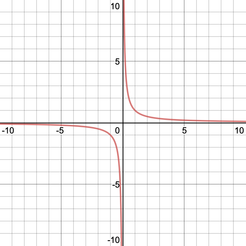
A third type of discontinuity is the so-called infinite discontinuity. Infinite discontinuities exist at points where the values of a function diverge to infinity. A classic example of an infinite discontinuity is the point

x = 0

for the function

f (x) = \frac{1}{x};

you can see the behavior of the infinite discontinuity in the graph of

y = f (x)

in Figure 1.4.3.

🔗
Figure 1.4.3. A plot of the function $y = f (x)$ for the function $f (x) = \frac{1}{x} .$

🔗

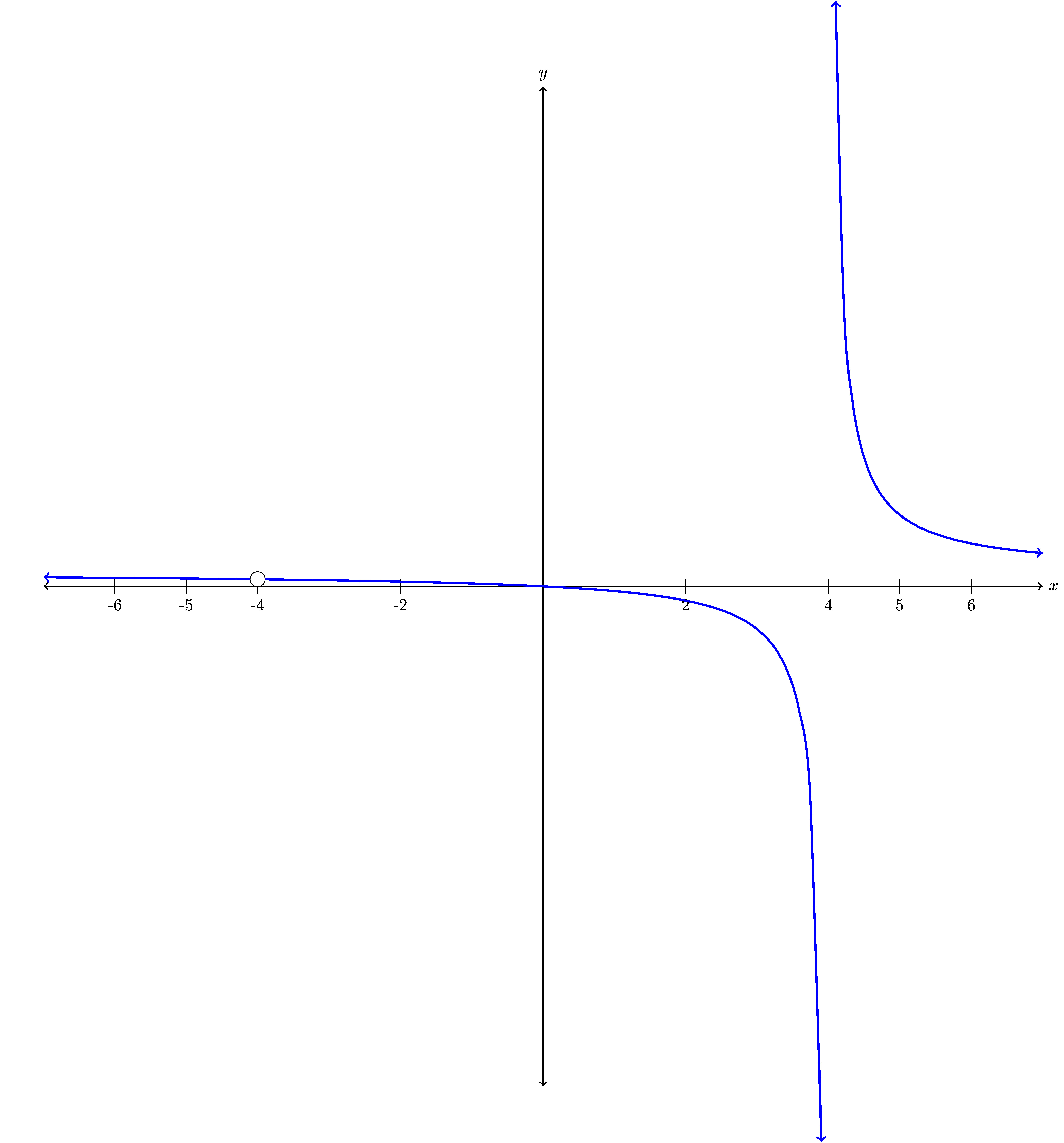
The graph below demonstrates the three types of discontinuity listed above: removable, jump, and infinite discontinuity.

🔗
Figure 1.4.4. Infinite discontinuity at $x = - 4,$ removable discontinuity at $x = - 1,$ and jump discontinuity at $x = 2 .$

🔗

Subsection 1.4.2 Limits and Continuity

🔗

Using limits, we can formalize the idea of continuity. Let us start by re-examining our first example given in Figure 1.4.1.

🔗

Consider the function in the left-most graph of Figure 1.4.1. We noted that

f (1)

is not defined, or

f (1) = D N E,

thus

f

is not continuous at $c = 1$ . For the function

g,

we observe that while

lim_{x \to 1} g (x) = 3,

the value of

g (1)

2,

and thus the limit does not equal the function value. Here, too, we will say that

g

is not continuous, even though the function is defined at

c = 1 .

Finally, the function

h

appears to be the most well-behaved of all three, since at

c = 1

its limit and its function value agree. That is,

lim_{x \to 1} h (x) = 3 = h (1) .

🔗

With no hole or jump in the graph of

h

c = 1,

we say that

h

is continuous there.

🔗

In Figure 1.4.2 we have what we called a jump discontinuity. Note that at the location of each jump:

lim_{x \to c^{-}} y \neq lim_{x \to c^{+}} y,

🔗

thus at each point that the graph of had a jump the

lim_{x \to c} y = D N E .

🔗

Similarly in Figure 1.4.3 we noted that the function was discontinuous at

x = 0

again

lim_{x \to 0^{-}} f (x) \neq lim_{x \to 0^{+}} f (x),

🔗

thus the

lim_{x \to 0} f (x) = D N E .

🔗

From these three examples we see that in order for a function to be continuous we need the limit to exist at the point. More formally, we make the following definition.

🔗

Continuous Function.

🔗

A function

f

is continuous at

x = c

provided that

$f$ has a limit as $x \to c,$
$f$ is defined at $x = c,$ and
$lim_{x \to c} f (x) = f (c) .$

🔗

Conditions (a) and (b) are technically contained implicitly in (c), but we state them explicitly to emphasize their individual importance. The definition says that a function is continuous at

x = c

provided that its limit as

x \to c

exists and equals its function value at

x = c .

Applying this definition to the types of discontinuities we have looked we can observe the following:

If the graph of a function has a hole at $x = a$ then $f (a) = D N E .$
If the graph of a function has an asymptote at $x = a$ then $f (a) = D N E$ or $lim_{x \to a} f (x) = D N E .$
If the graph of a function has an jump at $x = a$ then $lim_{x \to a} f (x) = D N E .$
If the graph of a function has a hole with a value at another y-value at $x = a$ then $lim_{x \to a} f (x) \neq f (a) .$

🔗

Continuous Function.

🔗

A function is said to be continuous on an interval

[a, b]

if the

lim_{x \to c} f (x) = f (c)

at every point

x = c

on the interval. That is, the function has no points of discontinuity on that interval.

🔗

Note: A function is continuous if nearby values of the independent variable give nearby values of the function. In practical work, continuity is important because it means that small errors in the independent variable lead to smalls errors in the function.

🔗

If a function is continuous at every point in an interval

[a, b],

we say the function is “continuous on

[a, b] .

” If a function is continuous at every point in its domain, we simply say the function is “continuous.” Thus we note that continuous functions are particularly nice: to evaluate the limit of a continuous function at a point, all we need to do is evaluate the function.

🔗

For example, consider

p (x) = x^{2} - 2 x + 3 .

It can be proved that every polynomial is a continuous function at every real number, and thus if we would like to know

lim_{x \to 2} p (x),

we simply compute

lim_{x \to 2} (x^{2} - 2 x + 3) = 2^{2} - 2 \cdot 2 + 3 = 3 = p (2) .

🔗

This route of substituting an input value to evaluate a limit works whenever we know that the function being considered is continuous. Besides polynomial functions, all exponential functions and the sine and cosine functions are continuous at every point, as are many other familiar functions and combinations thereof.

Example 1.4.5.

Consider the function

f (x) = \frac{3 x (x + 4)}{x^{2} - 16} .

Are there

x

-values where the function is discontinuous? If so, how do those

x

-values fail the limit definition of continuity?

Hint.

Consider the graph of

y = f (x) .

Figure 1.4.6. A plot of the function $y = f (x) .$

Answer.

f (x)

is discontinuous at

x = 4, - 4 .

At both points

f (4) = D N E

and

f (- 4) = D N E .

Also

lim_{x \to 4} f (x) = D N E .

Solution.

We first consider a graph of

y = f (x),

shown below.

Figure 1.4.7. A plot of the function $y = f (x) .$

Visual inspection of the graph certainly indicates discontinuities. However, we can make our visual inspection more precise through a little algebra. We start by expanding the numerator and denominator of the function. Specifically, we have

f (x) = \frac{3 x (x + 4)}{x^{2} - 16} = \frac{3 x (x + 4)}{(x + 4) (x - 4)} .

From here we see that there are two

x

-values at which the function is undefined: at

x = - 4, 4,

that is

f (x) = D N E

at these points hence the function is not continuous.

Note: Rational functions can be a challenging topic. For a more complete discussion of rational functions we refer the reader to Short-Run Behavior of Rational Functions

mathbooks.unl.edu/PreCalculus/Graphing-Rational-Functions.html

🔗

Subsection 1.4.3 Piecewise Functions

🔗

In many cases a simple function like

f (x) = x^{2}

may not fully describe the behavior of a phenomenon. In some of these cases we can turn to piecewise functions to give us the tools we need.

Example 1.4.8.

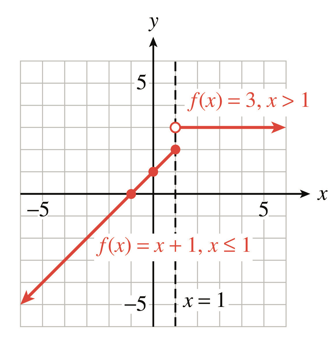
Is the function

f (x),

defined below, continuous at

x = 1,

use the limit to argue your answer

f (x) = {\begin{cases} x + 1 & if x \leq 1 \\ 3 & if x > 1 \end{cases} .

Hint.

Consider the graph of

f (x)

described in detail following the image — Figure 1.4.9.

Answer.

The function

f (x)

is not continuous since the

lim_{x \to 1} f (x) = D N E .

Solution.

For a piecewise function we must examine the point where the function changes. To do so we will examine the right and left hand limits. Here we use the fact that to the left of 1, that is

x < 1

the function is defined as

f (x) = x + 1 .

To the right of 1, that is

x > 1

the function is defined as

f (x) = 3 .

Thus:

lim_{x \to 1^{-}} f (x) = lim_{x \to 1^{-}} x + 1 = 1 + 1 = 2

lim_{x \to 1^{+}} f (x) = lim_{x \to 1^{+}} 3 = 3 .

Since the two sides are not the same

lim_{x \to 1} f (x) = D N E .

So the function

f (x)

is not continuous at

x = 1 .

🔗

The jumps that a piecewise function possesses make piecewise functions a natural place in which to explore continuity.

Example 1.4.10.

Is the function

h (x),

defined below, continuous for all values of

x

h (x) = {\begin{cases} 4 x^{2} & if x \leq 2 \\ 5 x + 6 & if x > 2 \end{cases}

Hint.

Consider the limit from the left and the limit from the right at

x = 2 .

Answer.

The function

h (x)

is continuous on the interval

(- \infty, \infty),

that is for all values of

x .

Solution.

For a piecewise function we must examine the point where the function changes. To do so we will examine the right and left hand limits. Here we use the fact that to the left of 2, that is

x < 2

the function is defined as

h (x) = 4 x^{2} .

To the right of 2, that is

x > 2

the function is defined as

h (x) = 5 x + 6 .

Thus:

lim_{x \to 2^{-}} h (x) = lim_{x \to 2^{-}} 4 x^{2} = 4 (2)^{2} = 16

lim_{x \to 2^{+}} h (x) = lim_{x \to 2^{+}} 5 x + 6 = 5 (2) + 6 = 16 .

Since the two sides are the same

lim_{x \to 2} h (x) = 16 .

So the function

h (x)

is continuous at

x = 2,

and since each piece is a polynomial this function is continuous on the interval

(- \infty, \infty),

that is for all values of

x .

🔗

Not only can we ask questions about when a piecewise function is continuous but we can also ask questions about how to make a piecewise function continuous by varying parameters.

Example 1.4.11.

Consider the piecewise function

D (x) = {\begin{cases} 4 x^{2} - k & if x < 2, \\ k x + 1 & if x \geq 2. \end{cases}

Find the value of

k

to make this function continuous for all

x .

Hint.

Consider the limit from the left and the limit from the right at

x = 2 .

Answer.

k = 5

Solution.

To determine a value of

k

to make

D (x)

continuous we will examine the right and left hand limits at

x = 2 .

Here we use the fact that to the left of 2, that is

x < 2

the function is defined as

D (x) = 4 x^{2} - k .

To the right of 2, that is

x > 2

the function is defined as

D (x) = k x + 1 .

Thus:

lim_{x \to 2^{-}} D (x) = lim_{x \to 2^{-}} 4 x^{2} - k = 4 (2)^{2} - k = 16 - k

lim_{x \to 2^{+}} D (x) = lim_{x \to 2^{+}} k x + 1 = k (2) + 1 = 2 k + 1 .

In order for

D (x)

to be continuous need the two sides to be equal, thus set them equal and solve for

k .

16 - k = 2 k + 1 .

15 = 3 k .

So the function

D (x)

is continuous at

x = 2

when

k = 5 .

Example 1.4.12.

Determine if each of the functions below is continuous at

x = 2 .

$f (x) = \ln (3 - x) .$
$g (x) = \frac{1}{x - 2} .$
$h (x) = {\begin{cases} x^{2} + 1 & if x \neq 2, \\ 3 & if x = 2. \end{cases}$

Hint.

Consider evaluating limits on each side and comparing that value to the value of the function at the point.

Answer.

$f$ is continuous at $x = 2 .$
$g$ is not continuous at $x = 2 .$
$h$ is not continuous at $x = 2 .$

Solution.

For each of these functions, we want to check that the limit exists at

x = 2,

the function is defined at

x = 2,

and these two values match.

We can examine the graph of $y = f (x)$ at $x = 2$ or examine function values nearby $x = 2$ on the left and right to find that $lim_{x \to 2} f (x) = 0 .$ Evaluating $f (2) = \ln (3 - 2) = \ln (1) = 0 .$ Thus, $lim_{x \to 2} f (x) = f (2),$ and $f$ is continuous at $x = 2 .$
Notice that the graph of $g$ has a vertical asymptote at $x = 2,$ so $g (2)$ is undefined. Hence, $g$ is not continuous at $x = 2 .$
For values of $x$ near 2 (from the left and right), we have $h (x)$ getting close to 5. Therefore, $lim_{x \to 2} h (x) = 5 .$ However, $h (2) = 3 .$ Since $lim_{x \to 2} h (x) \neq h (2),$ $h$ is not continuous at $x = 2 .$

🔗

Subsection 1.4.4 Properties of Limits and Continuous Functions

🔗

There are several properties of limits and continuous functions that are useful to have in your toolbox. Specifically, limits and continuous functions behave well under typical mathematical operations. While these properties can be proven in detail, we proceed to only state the properties.

🔗

Properties of Limits.

🔗

Assuming all the limits on the right-hand side exist:

If $b$ is a constant, then $lim_{x \to c} (b f (x)) = b (lim_{x \to c} f (x))$
$lim_{x \to c} (f (x) + g (x)) = lim_{x \to c} f (x) + lim_{x \to c} g (x)$
$lim_{x \to c} (f (x) \cdot g (x)) = lim_{x \to c} f (x) \cdot lim_{x \to c} g (x)$
$lim_{x \to c} (\frac{f (x)}{g (x)}) = \frac{lim_{x \to c} f (x)}{lim_{x \to c} g (x)},$ provided $lim_{x \to c} g (x) \neq 0$
For any constant $k,$ $lim_{x \to c} k = k$
$lim_{x \to c} x = c$

Example 1.4.13.

We can use algebra to compute

lim_{x \to 1} x^{2} (x^{3} + 2) .

Specifically,

\begin{aligned} lim_{x \to 1} x^{2} (x^{3} + 2) & = (lim_{x \to 1} x^{2}) (lim_{x \to 1} (x^{3} + 2)) \\ = (lim_{x \to 1} x^{2}) (lim_{x \to 1} x^{3} + lim_{x \to 1} 2) \\ = 1 (1 + 2) \\ = 3. \end{aligned}

🔗

Continuity of Sums, Products, and Quotients of Functions.

🔗

Suppose that

f

and

g

are continuous on an interval and that

b

is a constant. Then, on that same interval,

$b f (x)$ is continuous.
$f (x) + g (x)$ is continuous.
$f (x) g (x)$ is continuous.
$\frac{f (x)}{g (x)}$ is continuous, provided $g (x) \neq 0$ on the interval.

🔗

Continuity of Composite Functions.

🔗

f

and

g

are continuous, and if the composite function

f (g (x))

is defined on an interval, then

f (g (x))

is continuous on that interval.

🔗

Subsection 1.4.5 Summary of Limits and Continuity

🔗

The concepts discussed in the last two sections will be important in later sections. The following is a short summary of these sections and an example that ties together the concepts of limits and continuity.

For a function $f$ defined on an interval around a number $c,$
$lim_{x \to c} f (x) = L$
means that the value of $f (x)$ gets as close as we want to a number $L$ whenever $x$ is sufficiently close to $c,$ assuming the value $L$ exists.
We define a limit from the left and a limit from the right in the same way as above, while adding the stipulation that $x < c$ for the left limit and $x > c$ for the right limit. That is, as we move $x$ sufficiently close to $c$ from the left on a number line ( $x < c$ ), $f (x)$ gets as close to the limit value as we want. Similarly for the limit from the right.
The one-sided limits help to determine if a limit exists as $x$ approaches a value $c .$ More specifically, $lim_{x \to c} f (x) = L$ if and only if $lim_{x \to c^{-}} f (x) = L = lim_{x \to c^{+}} f (x)$
Limits also help us determine the continuity of a function at a point $x = c .$ A function $f$ that has a limit as $x \to c,$ is defined at $x = c,$ and $lim_{x \to c} f (x) = f (c)$ is continuous at $x = c .$

Example 1.4.14.

In this example, we take a closer look at a function whose graph we previously encountered. For convenience, this graph is reproduced below in Figure 1.4.15.

At which values of $c$ does $lim_{x \to c} f (x)$ not exist?
At which values of $c$ is $f (c)$ not defined?
At which values of $c$ does $f$ have a limit, but $lim_{x \to c} f (x) \neq f (c) ?$
State all values of $c$ for which $f$ is not continuous at $x = c .$
Which condition is stronger, and hence implies the other: $f$ has a limit at $x = c$ or $f$ is continuous at $x = c ?$ Explain, and hence complete the following sentence: “If $f$ at $x = c,$ then $f$ at $x = c,$ ” where you complete the blanks with has a limit and is continuous, using each phrase once.

Hint.

Consider the left- and right-hand limits at each value.
Carefully examine places on the graph where there’s an open circle.
Are there locations on the graph where the function has a limit but there’s a hole in the graph?
Remember that at least one of three conditions must fail: if the function lacks a limit, if the function is undefined, or if the limit exists but does not equal the function value, then $f$ is not continuous at the point.
Note that the definition of being continuous requires the limit to exist.

Answer.

$c = - 2;$ $c = + 2 .$
$c = 3 .$
$c = - 1;$ $c = 3 .$
$c = - 2;$ $c = 2;$ $c = 3;$ $c = - 1 .$
“If $f$ is continuous at $x = c,$ then $f$ has a limit at $x = c .$ ”

Solution.

$lim_{x \to c} f (x)$ does not exist at $c = - 2$ since

$lim_{x \to - 2^{-}} f (x) = 2 \neq - 1 = lim_{x \to - 2^{+}},$

and $lim_{x \to c} f (x)$ does not exist at $c = 2$ since $lim_{x \to 2^{+}} f (x)$ does not exist due to the infinitely oscillatory behavior of $f .$
The only point at which $f$ is not defined is at $c = 3 .$
At $c = - 1,$ note that $lim_{x \to - 1} f (x)$ exists (and appears to have value approximately $- 3.25$ ), but $f (- 1) = 1$ and thus $lim_{x \to - 1} f (x) \neq f (- 1) .$ At $c = 3,$ we have $lim_{x \to 3} f (x) = - 2.5,$ but $f (3)$ is not defined so the limit exists but does not equal the function value.
Based on our work in (a), (b), and (c), $f$ is not continuous at $c = - 2$ and $c = 2$ because $f$ does not have a limit at those points; $f$ is not continuous at $c = 3$ since $f$ is not defined there; and $f$ is not continuous at $c = - 1$ because at that point its limit does not equal its function value.
“If $f$ is continuous at $x = c,$ then $f$ has a limit at $x = c,$ ” since one of the defining properties of “being continuous” at $x = c$ is that the function has a limit at that input value. This shows that being continuous is a stronger condition than having a limit.

🔗

Exercises 1.4.6 Exercises

🔗

1. Types of discontinuity.

🔗

Determine the point at which the function

f (x) = \frac{1}{x - 2}

is discontinuous and state the type of discontinuity: removable, jump, infinite, or none of these.

🔗

x =

🔗

Choose the type

🔗

2. Types of discontinuity.

🔗

Determine the points at which the function is discontinuous and state the type of discontinuity: removable, jump, infinite, or none of these.

🔗

f (x) = \frac{x - 2}{∣ x - 1 ∣}

🔗

x =

🔗

Choose the type

🔗

3. Types of discontinuity.

🔗

Enter T or F depending on whether the statement is true or false. (You must enter T or F -- True and False will not work.)

🔗

The function $f (t) = \frac{1}{t^{2} - t}$ has an infinite discontinuity at $t = 1 .$

🔗

4. Determining continuity from a graph.

🔗

Answer the questions based on the graph of

y = f (x)

shown above.

🔗

If you are having a hard time seeing the picture clearly, click on the picture. It will expand to a larger picture on its own page so that you can inspect it more clearly.

🔗

f

is
is not

🔗

continuous at

- 2 .

🔗

f

is
is not

🔗

continuous at

- 1 .

🔗

f

is
is not

🔗

continuous at

0 .

🔗

f

is
is not

🔗

continuous at

1 .

🔗

f

is
is not

🔗

continuous at

3 .

🔗

f

is
is not

🔗

continuous at

4 .

🔗

5. Determining continuity from a graph.

🔗

Answer the questions based on the graph of

y = f (x)

shown above.

🔗

If you are having a hard time seeing the picture clearly, click on the picture. It will expand to a larger picture on its own page so that you can inspect it more clearly.

🔗

f

is
is not

🔗

continuous at

0 .

🔗

f

is
is not

🔗

continuous at

1 .

🔗

f

is
is not

🔗

continuous at

2 .

🔗

6. Interpretting continuity.

🔗

An electrical circuit switches instantaneously from a 6 volt battery to a 21 volt battery 7 seconds after being turned on. Sketch on a sheet of paper a graph the battery voltage against time. Then fill in the formulas below for the function represented by your graph.

🔗

For