Kevin Gonzales, Eric Hopkins, Catherine Zimmitti, Cheryl Kane, Modified to fit Applied Calculus from Coordinated Calculus by Nathan Wakefield et. al., Based upon Active Calculus by Matthew Boelkins
Section5.3The Definite Integral
Motivating Questions
How does increasing the number of subintervals affect the accuracy of the approximation generated by a Riemann sum?
What is the definition of the definite integral of a function \(f\) over the interval \([a,b]\text{?}\)
What does the definite integral measure exactly, and what are some of the key properties of the definite integral?
In Section5.2, we introduced the definite integral \(\displaystyle \int\limits_a^b f(x) dx\text{.}\)
The definite integral of a continuous function \(f\) on the interval \([a,b]\text{,}\) denoted \(\displaystyle \int\limits_a^b f(x) \, dx\text{,}\) is the real number given by
where \(\Delta x = \frac{b-a}{n}\text{,}\) \(x_i = a + i\Delta x\) (for \(i = 0, \ldots, n\)), and \(x_i^*\) satisfies \(x_{i-1} \le x_i^* \le x_i\) (for \(i = 1, \ldots, n\)).
We call the values \(a\) and \(b\) the limits of integration. The process of determining the real number \(\displaystyle \int\limits_a^b f(x) \, dx\) is called evaluating the definite integral.
While there are several different interpretations of the definite integral, for now the most important is that \(\displaystyle \int\limits_a^b f(x) \, dx\) measures the net signed area bounded by \(y = f(x)\) and the \(x\)-axis on the interval \([a,b]\text{.}\)
For example, if \(f\) is the function pictured in Figure5.44, and \(A_1\text{,}\) \(A_2\text{,}\) and \(A_3\) are the exact areas bounded by \(f\) and the \(x\)-axis on the respective intervals \([a,b]\text{,}\) \([b,c]\text{,}\) and \([c,d]\text{,}\) then
Figure5.46A continuous function \(f\) on the interval \([a,d]\text{.}\)
To compute the value of a definite integral from the definition, we have to take the limit of a sum. While this is possible to do in select circumstances, it is also tedious and time-consuming. Luckily, we have a very useful theorem, called the fundamental theorem of calculus, which tells us how to compute a definite integral of a continuous function.
SubsectionThe Fundamental Theorem of Calculus
Fundamental Theorem of Calculus
If \(f(x)\) is a continuous function on \([a,b]\text{,}\) and \(F\) is any antiderivative of \(f(x)\text{,}\) then \(\displaystyle \int\limits_a^b f(x) \, dx = F(b) - F(a)\text{.}\)
A common alternate notation for \(F(b) - F(a)\) is
where we read the righthand side as the function \(F\) evaluated from \(a\) to \(b\text{.}\) In this notation, the FTC (fundamental theorem of calculus) says that
The value of the FTC is that is allows us to compute the definite integral using the rules that we found in Section5.1. For instance since \(\frac{d}{dx}[\frac{1}{3}x^3] = x^2\text{,}\) the FTC tells us that
In general finding an antiderivative can be far from simple; it is often difficult or even impossible. While we can differentiate just about any function, even some relatively simple functions don't have an elementary antiderivative. A significant portion of integral calculus (which is the main focus of second semester college calculus) is devoted to the problem of finding antiderivatives. For now we will focus only on applying the rules that we found in Section5.1 to definite integrals.
Example5.47
Use the Fundamental Theorem of Calculus (FTC) and the rules developed in Section5.1 to evaluate the following integral:
Second, we plug in the bounds of integration, always plugging in the top value to every \(x\) first and subtract plugging in the bottom value to every \(x\text{.}\)
\(\bf{Note}:\) it is very important to have parentheses around the each term, especially the second so the minus sign distributes to every term. Thus:
First use the FTC and apply the power rule, constant rule, and sum and difference rule from Section5.1. Second, plug in the bounds appropriately to get:
First use the FTC and apply the Natural Log, Exponential rule, constant rule, and sum and difference rule from Section5.1. Second, plug in the bounds appropriately to get:
As we saw from Section5.2, the definite integral \(\displaystyle \int\limits_a^b f(x) dx\) gives the exact area under the curve \(f(x)\) on the interval \([a,b]\text{.}\)
Example5.50
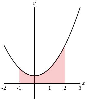
Find the exact area under the curve \(f(x)=x^2+1\) on the interval \([-1,2]\text{,}\) shown below. Figure5.51Area under the curve \(f(x)=x^2+1\text{.}\)
We can also use definite integrals to express the change in position and the distance traveled by a moving object. If \(v\) is a velocity function on an interval \([a,b]\text{,}\) then the change in position of the object, \(s(b) - s(a)\text{,}\) is given by
If the velocity function is nonnegative on \([a,b]\text{,}\) then \(\int\limits_a^b v(t) \,dt\) tells us the total distance the object traveled. If the velocity is sometimes negative on \([a,b]\text{,}\) we can use definite integrals to find the areas bounded by the function on each interval where \(v\) does not change sign, and the sum of these areas will tell us the distance the object traveled.
The total distance traveled given the velocity is not the only total change that we can compute using a definite integral.
Total Change Theorem
If \(f\) is a continuously differentiable function on \([a,b]\) with derivative \(f'\text{,}\) then \(\displaystyle f(b) - f(a) = \int\limits_a^b f'(x) \, dx\text{.}\) That is, the definite integral of the rate of change of a function on \([a,b]\) is the total change of the function itself on \([a,b]\text{.}\)
The Total Change Theorem enables us to answer questions about a function whose rate of change we know.
Example5.52
A company finds that the marginal profit, in dollars per foot, from drilling a well that is \(x\) feet deep is given by
\begin{equation*}
P'(x)=4x^{1/6}
\end{equation*}
Find the total profit from drilling a well that is \(130\) feet deep.
In this example we use the Total Change Theorem: since we are given the marginal profit, \(P'(x)\text{,}\) we can integrate from \([0,130]\) to find the total profit.
To find the total accumulated sales from the \(2^{nd}\) day through the \(10^{th}\) day again we need to integrate. Here we must be careful with our bounds. The 2nd day starts when the first day ends, thus we must integrate from \(x=1\text{,}\) the end of the first day, to \(x=10\text{.}\) So the total accumulated sales are
Although this is not given as a derivative, we are still given a rate of change. Thus, we can again apply the Total Change Theorem here to find the total amount of cars that pass by the point. We must determine the bounds of integration, here \(t=0\) is 8am and since we want to go from 8am to 10 am, which is 2 hours later, the bounds are \(t=0\) to \(t=2\text{.}\) Thus
Suppose that pollutants are leaking out of an underground storage tank at a rate of \(r(t)\) gallons/day, where \(t\) is measured in days. It is conjectured that \(r(t)\) is given by the formula \(r(t) = 0.0069t^3 -0.125t^2+11.079\) over a certain 12-day period. The graph of \(y=r(t)\) is given in Figure5.56. What is the meaning of \(\displaystyle \int\limits_4^{10} r(t) \, dt\) and what is its value? What is the average rate at which pollutants are leaving the tank on the time interval \(4 \le t \le 10\text{?}\)
Figure5.56The rate \(r(t)\) of pollution leaking from a tank, measured in gallons per day.
Since \(r(t) \ge 0\text{,}\) the value of \(\displaystyle \int\limits_4^{10} r(t) \, dt\) is the area under the curve on the interval \([4,10]\text{.}\) A Riemann sum for this area will have rectangles with heights measured in gallons per day and widths measured in days, so the area of each rectangle will have units of
Thus, the definite integral tells us the total number of gallons of pollutant that leak from the tank from day 4 to day 10. The Total Change Theorem tells us the same thing: if we let \(R(t)\) denote the total number of gallons of pollutant that have leaked from the tank up to day \(t\text{,}\) then \(R'(t) = r(t)\text{,}\) and
the number of gallons that have leaked from day 4 to day 10.
To compute the exact value of the integral, we use the Fundamental Theorem of Calculus. Antidifferentiating \(r(t) = 0.0069t^3 -0.125t^2+11.079\text{,}\) we find that
Thus, approximately 44.282 gallons of pollutant leaked over the six day time period.
To find the average rate at which pollutant leaked from the tank over \(4 \le t \le 10\text{,}\) we compute the average value of \(r\) on \([4,10]\text{.}\) Thus,
During a 40-minute workout, a person riding an exercise machine burns calories at a rate of \(c\) calories per minute, where the function \(y = c(t)\) is given in Figure5.58. On the interval \(0 \le t \le 10\text{,}\) the formula for \(c\) is \(c(t) = -0.05t^2 + t + 10\text{,}\) while on \(30 \le t \le 40\text{,}\) its formula is \(c(t) = -0.05t^2 + 3t - 30\text{.}\)
Figure5.58The rate \(c(t)\) at which a person exercising burns calories, measured in calories per minute.
What is the exact total number of calories the person burns during the first 10 minutes of her workout?
Let \(C(t)\) be an antiderivative of \(c(t)\text{.}\) What is the meaning of \(C(40) - C(0)\) in the context of the person exercising? Include units in your answer.
Since the units on a rectangle in a Riemann sum are cal/min for the height and min for the width, the units of the area of such a rectangle are calories, and hence the units of area under the curve \(y = c(t)\) are given in total calories. Hence, the total calories burned during the first 10 minutes of the workout is given by the definite integral \(\int\limits_0^{10} c(t) \, dt\text{.}\) We use the FTC and evaluate the integral, finding that
and therefore, as discussed in (a), the meaning of this value is the total calories burned on \([0,40]\text{.}\)
SubsectionSummary
The limit of Riemann sums can often be tricky to compute. Luckily, we have the fundamental theorem of calculus, often abbreviated FTC, which tells us that if \(f'(x) \) is a continuous function on \([a,b] \text{,}\) and \(f \) is any antiderivative of \(f' \text{,}\) then
So, to compute the definite integral, we need to find an antiderivative of \(f'\text{,}\) evaluate at the endpoints of the interval, and compute the difference.
The total change theorem tells us that the definite integral of the rate of change of a function on \([a,b] \) is the total change of the function itself on \([a,b] \text{.}\) In the setting where we consider the integral of a velocity function \(v\text{,}\) \(\int_a^b v(t) \,dt\) measures the exact change in position of the moving object on \([a,b]\text{;}\) when \(v\) is nonnegative, \(\int_a^b v(t) \,dt\) is the object's distance traveled on \([a,b]\text{.}\)