Kevin Gonzales, Eric Hopkins, Catherine Zimmitti, Cheryl Kane, Modified to fit Applied Calculus from Coordinated Calculus by Nathan Wakefield et. al., Based upon Active Calculus by Matthew Boelkins
Section5.2Determining Area Under a Curve
Motivating Questions
If we know the velocity of a moving body at every point in a given interval, can we determine the distance the object has traveled on that time interval?
How is the problem of finding distance traveled related to finding the area under a certain curve? If velocity is negative, how does this impact the problem of finding distance traveled?
What are Riemann sums, and how can they be used to estimate the area under the any continuous curve?
We saw in Section5.1 how to find the antiderivative of a function. In this section we explore how the antiderivative of a function is connected to the area under the curve of the function. To understand this, we will start with a more specific question: if we know the instantaneous velocity of an object moving along a straight line path, can we find its corresponding position function?
Example5.13
Suppose that a person is taking a walk along a long straight path and walks at a constant rate of 3 miles per hour.
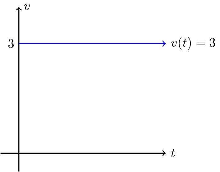
Sketch and label a graph of the velocity function \(v(t) = 3\text{.}\)
How far did the person travel during the two hours? How is this distance related to the area of a certain region under the graph of \(y = v(t)\text{?}\)
Find an algebraic formula, \(s(t)\text{,}\) for the position of the person at time \(t\text{,}\) assuming that \(s(0) = 0\text{.}\) Explain your thinking.
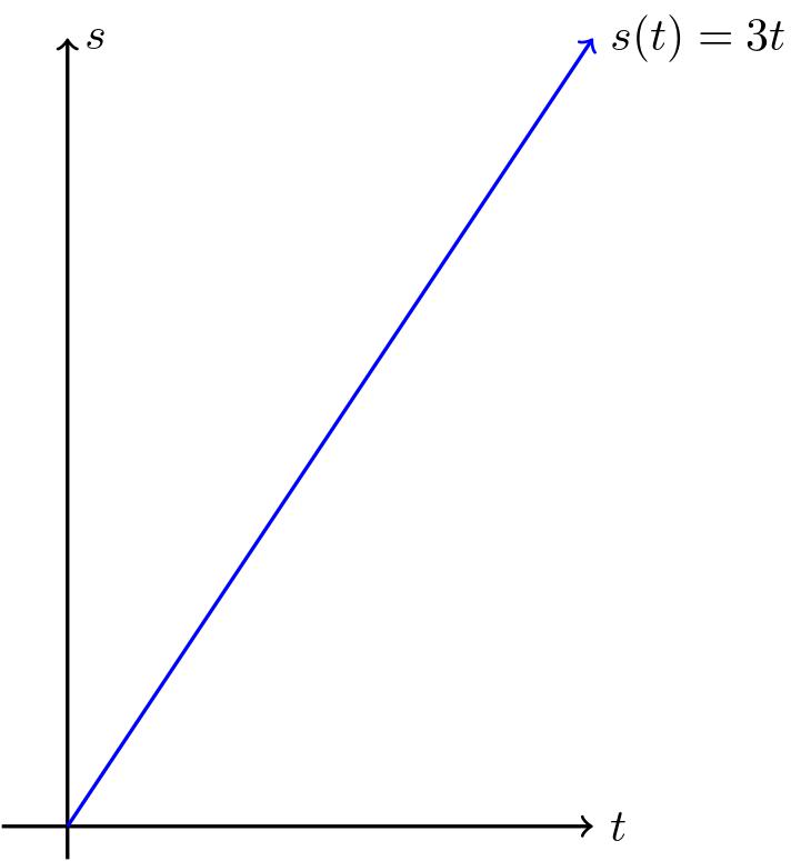
Sketch a labeled graph of the position function \(y = s(t)\text{.}\)
For what values of \(t\) is the position function \(s\) increasing? Explain why this is the case using relevant information about the velocity function \(v\text{.}\)
Figure5.16The velocity is constant, which creates a horizontal line.
If the person is traveling at a constant speed of 3 miles per hour, we can find the distance traveled by multiplying the speed by the amount of time they are walking. So, the person traveled 6 miles in 2 hours.
The height of the function is always at 3 and the time is given by the \(x\)-axis. The distance traveled is the same as the area under the curve of \(v(t)\) between 0 and 2.
For every time, the position is given by multiplying the constant velocity, 3, by the time. Therefore, \(s(t)=3t\text{.}\)
Figure5.17The position function.
The position function \(s(t)\) is always increasing. This is because the velocity is constantly positive. We can see this also by looking at the graph of \(s(t)\text{,}\) which is a straight line with a positive slope.
SubsectionArea under the graph of the velocity function
In Example5.13, we learned that when the velocity of a moving object is constant (and positive), the area under the velocity curve over an interval of time tells us the distance the object traveled.
Figure5.18At left, a constant velocity function; at right, a non-constant velocity function.
The left-hand graph of Figure5.18 shows the velocity of an object moving at 2 miles per hour over the time interval \([1,1.5]\text{.}\) The area \(A_1\) of the shaded region under \(y = v(t)\) on \([1,1.5]\) is
This result is due to the formula for area of a rectangle, but it is also simply the fact that distance equals rate times time, provided the rate is constant. Thus, if \(v(t)\) is constant on the interval \([a,b]\text{,}\) the distance traveled on \([a,b]\) is equal to the area \(A\) given by
\begin{equation*}
A = v(a) (b-a) = v(a) \Delta t\text{,}
\end{equation*}
where \(\Delta t\) is the change in \(t\) over the interval. Since the velocity is constant, we can use any value of \(v(t)\) on the interval \([a,b]\text{,}\) we simply chose \(v(a)\text{,}\) the value at the interval's left endpoint. For several examples where the velocity function is piecewise constant, see http://gvsu.edu/s/9T.1Marc Renault, calculus applets.
The situation is more complicated when the velocity function is not constant. On relatively small intervals where \(v(t)\) does not vary much, we can use the area principle to estimate the distance traveled. The right-hand graph of Figure5.18 shows a non-constant velocity function. On the interval \([1,1.5]\text{,}\) the velocity varies from \(v(1) = 2.5\) down to \(v(1.5) \approx 2.1\text{.}\) One estimate for the distance traveled is the area of the pictured rectangle,
Note that because \(v\) is decreasing on \([1,1.5]\text{,}\) \(A_2 = 1.25\) is an over-estimate of the actual distance traveled.
To estimate the area under this non-constant velocity function on a wider interval, say \([0,3]\text{,}\) one rectangle will not give a good approximation. Instead, we could use the six rectangles pictured in Figure5.19, find the area of each rectangle, and add up the total. Obviously there are choices to make and issues to understand: How many rectangles should we use? Where should we evaluate the function to decide the rectangle's height? What happens if the velocity is sometimes negative? Can we find the exact area under any non-constant curve?
Figure5.19Using six rectangles to estimate the area under \(y = v(t)\) on \([0,3]\text{.}\)
We will study these questions and more in what follows; for now it suffices to observe that the simple idea of the area of a rectangle gives us a powerful tool for estimating distance traveled from a velocity function, as well as for estimating the area under an arbitrary curve. To explore the use of multiple rectangles to approximate area under a non-constant velocity function, see the applet found at http://gvsu.edu/s/9U.2Marc Renault, calculus applets.
Example5.20
Suppose that a person is walking in such a way that their velocity varies slightly according to the information given in Table5.21 and graph given in Figure5.22.
\(t\)
\(v(t)\)
\(0.00\)
\(1.500\)
\(0.25\)
\(1.789\)
\(0.50\)
\(1.938\)
\(0.75\)
\(1.992\)
\(1.00\)
\(2.000\)
\(1.25\)
\(2.008\)
\(1.50\)
\(2.063\)
\(1.75\)
\(2.211\)
\(2.00\)
\(2.500\)
Table5.21Velocity data for the person walking.Figure5.22The graph of \(y = v(t)\text{.}\)
Using the grid, graph, and given data, estimate the distance traveled by the walker during the two hour interval from \(t = 0\) to \(t = 2\text{.}\) You should use time intervals of width \(\Delta t = 0.5\text{.}\) Choose a way to use the function consistently to determine the height of each rectangle in order to approximate distance traveled.
How could you get a better approximation of the distance traveled on \([0,2]\text{?}\) Explain, and then find this new estimate.
Thus, \(D \approx 3.75\) miles. Note that you could have used used the function value at the right end of the interval, the midpoint of the interval, etc., as long as it is consistent for each rectangle.
Using 8 rectangles of width \(0.25\text{,}\) \(D \approx 3.875\text{.}\)
Using rectangles of width \(\Delta t = 0.5\) and choosing to set the heights of the rectangles from the function value at the left end of the interval, we see the following graph and find the sum of the areas of the rectangles to be
Thus, the distance traveled is approximately \(D \approx 3.75\) miles.
It appears that a better approximation could be found using narrower rectangles. If we move to 8 rectangles of width \(0.25\text{,}\) similar computations show that \(D \approx 3.875\text{.}\)
SubsectionWhen velocity is negative
Consider a simple example where a woman goes for a walk on the beach along a stretch of very straight shoreline that runs east-west. We assume that her initial position is \(s(0) = 0\text{,}\) and that her position function increases as she moves east from her starting location. For instance, \(s = 1\) mile represents one mile east of the start location, while \(s = -1\) tells us she is one mile west of where she began walking on the beach.
Now suppose she walks in the following manner. From the outset at \(t = 0\text{,}\) she walks due east at a constant rate of \(3\) mph for 1.5 hours. After 1.5 hours, she stops abruptly and begins walking due west at a constant rate of \(4\) mph and does so for 0.5 hours. Then, after another abrupt stop and start, she resumes walking at a constant rate of \(3\) mph to the east for one more hour. What is the total distance she traveled on the time interval from \(t = 0\) to \(t = 3\text{?}\) What the total change in her position over that time?
These questions are possible to answer without calculus because the velocity is constant on each interval. From \(t = 0\) to \(t = 1.5\text{,}\) she traveled
Since the velocity for \(1.5 \lt t \lt 2\) is \(v = -4\text{,}\) indicating motion in the westward direction, the woman first walked 4.5 miles east, then 2 miles west, followed by 3 more miles east. Thus, the total change in her position is
We have been able to answer these questions fairly easily, and if we think about the problem graphically, we can generalize our solution to the more complicated setting when velocity is not constant, and possibly negative.
Figure5.23At left, the velocity function of the person walking; at right, the corresponding position function.
In Figure5.23, we see how the distances we computed can be viewed as areas: \(A_1 = 4.5\) comes from multiplying rate times time (\(3 \cdot 1.5\)), as do \(A_2\) and \(A_3\text{.}\) But while \(A_2\) is an area (and is therefore positive), because the velocity function is negative for \(1.5 \lt t \lt 2\text{,}\) this area has a negative sign associated with it. The negative area distinguishes between distance traveled and change in position.
But the change in position has to account for travel in the negative direction. An area above the \(t\)-axis is considered positive because it represents distance traveled in the positive direction, while one below the \(t\)-axis is viewed as negative because it represents travel in the negative direction. Thus, the change in the woman's position is
In other words, the woman walks 4.5 miles in the positive direction, followed by 2 miles in the negative direction, and then 3 more miles in the positive direction.
Negative velocity is also seen in the graph of the position function \(y=s(t)\text{.}\) Its slope is negative (specifically, \(-4\)) on the interval \(1.5\lt t\lt 2\) because the velocity is \(-4\) on that interval. The negative slope shows the position function is decreasing because the woman is walking east, rather than west.
To summarize: we see that if velocity is sometimes negative, a moving object's change in position different from its distance traveled. If we compute separately the distance traveled on each interval where velocity is positive or negative, we can calculate either the total distance traveled or the total change in position. We assign a negative value to distances traveled in the negative direction when we calculate change in position, but a positive value when we calculate the total distance traveled.
Example5.24
Suppose that an object moving along a straight line path has its velocity \(v\) (in meters per second) at time \(t\) (in seconds) given by the piecewise linear function whose graph is pictured at left in Figure5.25. We view movement to the right as being in the positive direction (with positive velocity), while movement to the left is in the negative direction.
Figure5.25The velocity function of a moving object.
Suppose further that the object's initial position at time \(t = 0\) is \(s(0) = 1\text{.}\)
Determine the total distance traveled and the total change in position on the time interval \(0 \le t \le 2\text{.}\) What is the object's position at \(t = 2\text{?}\)
On what time intervals is the moving object's position function increasing? Why? On what intervals is the object's position decreasing? Why?
What is the object's position at \(t = 8\text{?}\) How many total meters has it traveled to get to this point (including distance in both directions)? Is this different from the object's total change in position on \(t = 0\) to \(t = 8\text{?}\)
Find the exact position of the object at \(t = 1, 2, 3, \ldots, 8\) and use this data to sketch an accurate graph of \(y = s(t)\) on the axes provided at right in Figure5.25. How can you use the provided information about \(y = v(t)\) to determine the concavity of \(s\) on each relevant interval?
Total distance traveled is \(2\text{;}\) change in position is \(0\text{.}\)
The position function is increasing on \(0 \lt t \lt 1\) and \(4 \lt t \lt 8 \) because the velocity is positive. The position function is decreasing on \(1 \lt t \lt 4 \) because the velocity is negative.
By finding the area of the triangular regions formed between \(y = v(t)\) and the \(t\)-axis on \([0,1]\) and \([1,2]\) (each of which is \(1\)), it follows that the object's total distance traveled is \(2\text{,}\) while its change in position is \(0\text{.}\) The latter is true since the net signed area bounded by \(v\) on \([0,2]\) is \(1 - 1 = 0\text{.}\)
The object's position is increasing wherever its velocity is positive, hence for \(0 \lt t \lt 1\) and \(4 \lt t \lt 8 \text{.}\) The object's position is decreasing wherever its velocity is negative, hence for \(1 \lt t \lt 4 \text{.}\)
By calculating the area bounded by the curve, we find 1 unit of area on \([0,1]\text{,}\) 4 units of area on \([1,4]\text{,}\) and 8 units of area on \([4,8]\text{,}\) thus the total distance traveled on \(0 \le t \le 8\) is \(D = 1 + 4 + 8\) meters. As the change in position is given by the net signed area on this interval, we find that the change in position is
In the figure below, at left we list all of the areas bounded by \(v\) on each one-unit subinterval. Along with the given starting point that \(s(0) = 1\text{,}\) we use the resulting changes in position to plot points for the function \(s\text{.}\) For instance, we know \(s(1) - s(0) = 1\text{,}\) hence \(s(1) = 2\text{.}\) Similarly, \(s(2) - s(1) = -1\text{,}\) thus \(s(2) = 1\text{.}\) Continuing across the interval, we generate the function \(s\) that is pictured at right. Note that the portion of \(s\) from \(t = 2\) to \(t = 3\) is linear because \(v\) is constant there, while the other parts of \(s\) appear to be quadratic, as they correspond to intervals where \(v\) is linear.
SubsectionLeft and Right Hand Sums
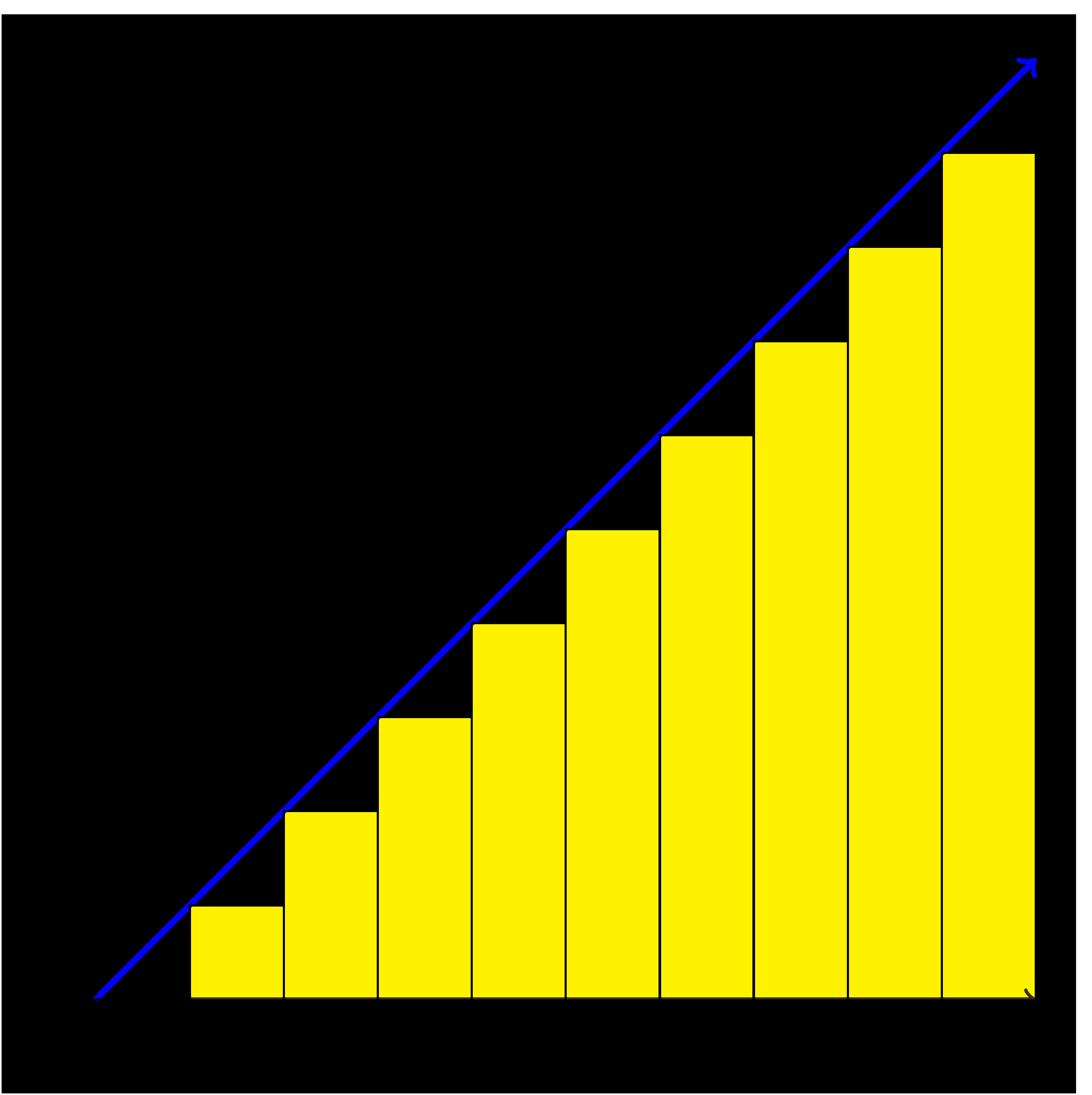
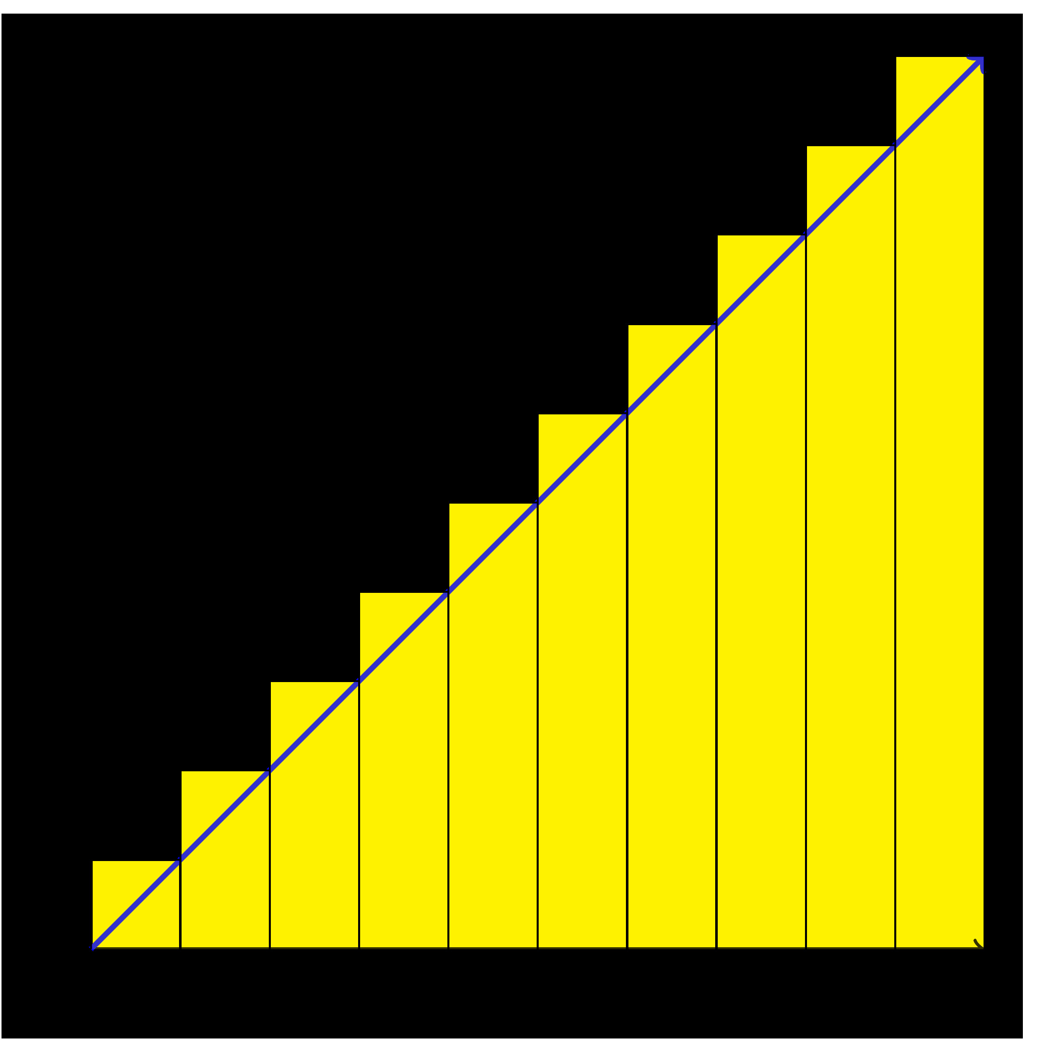
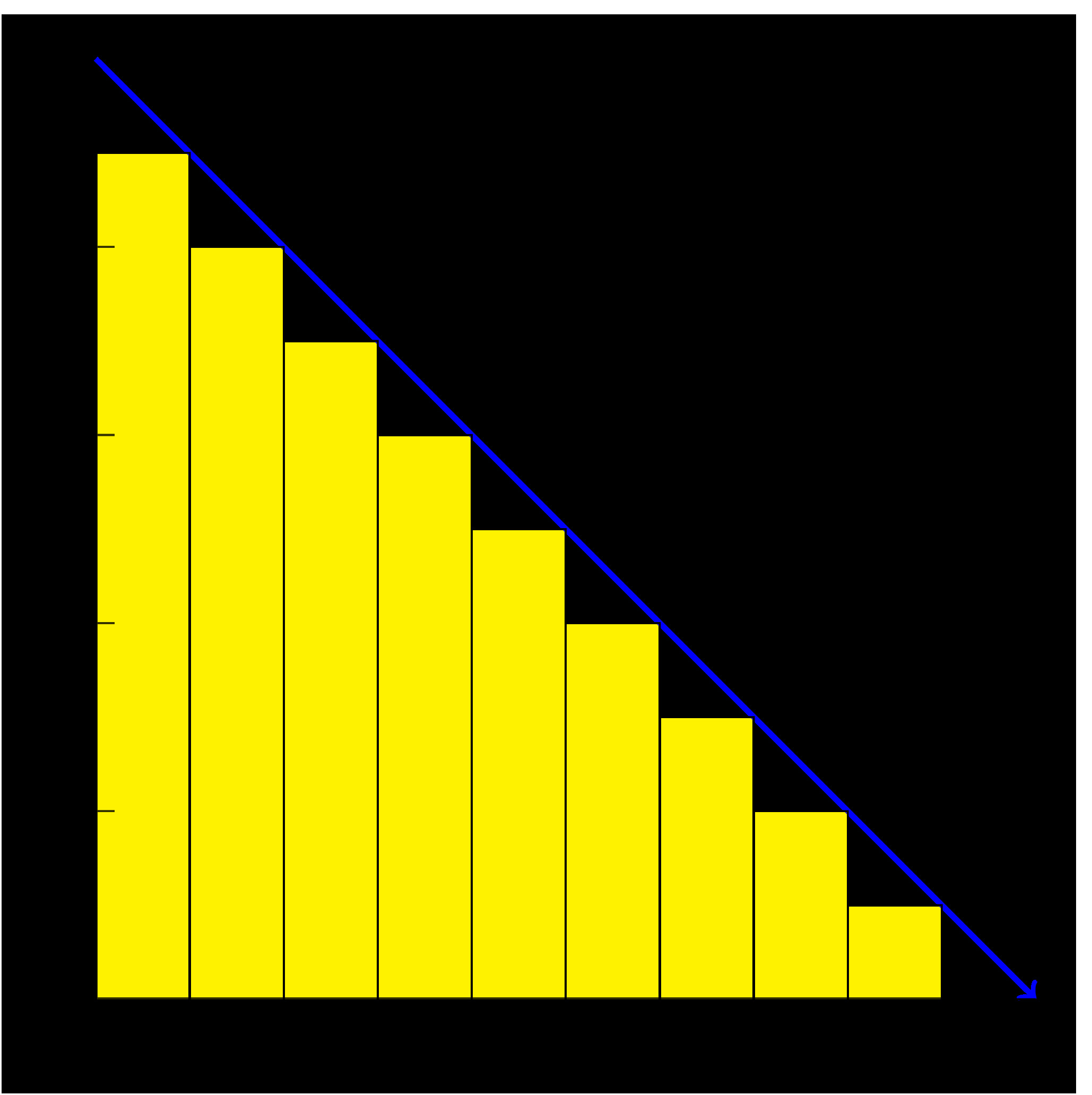
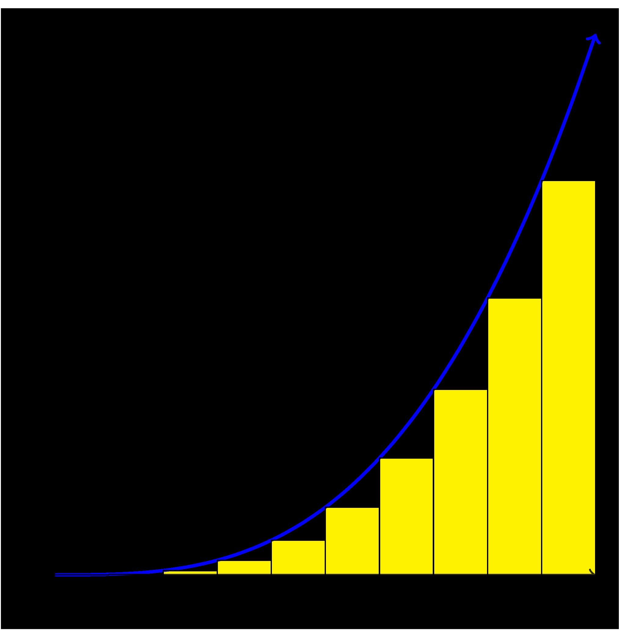
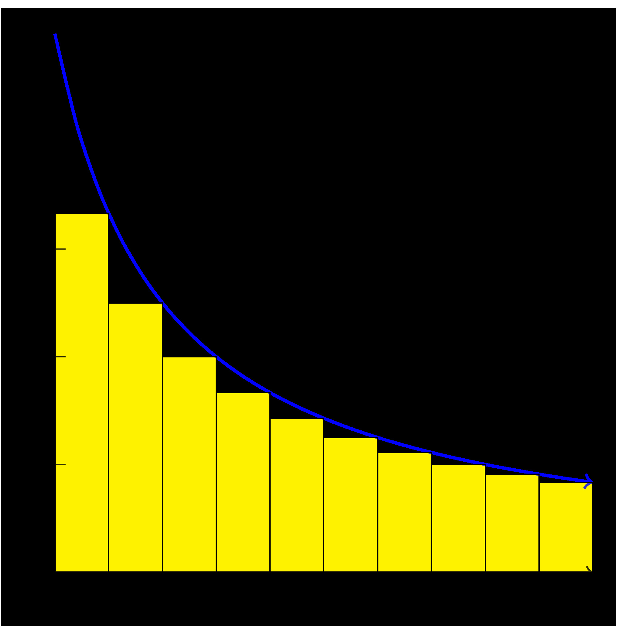
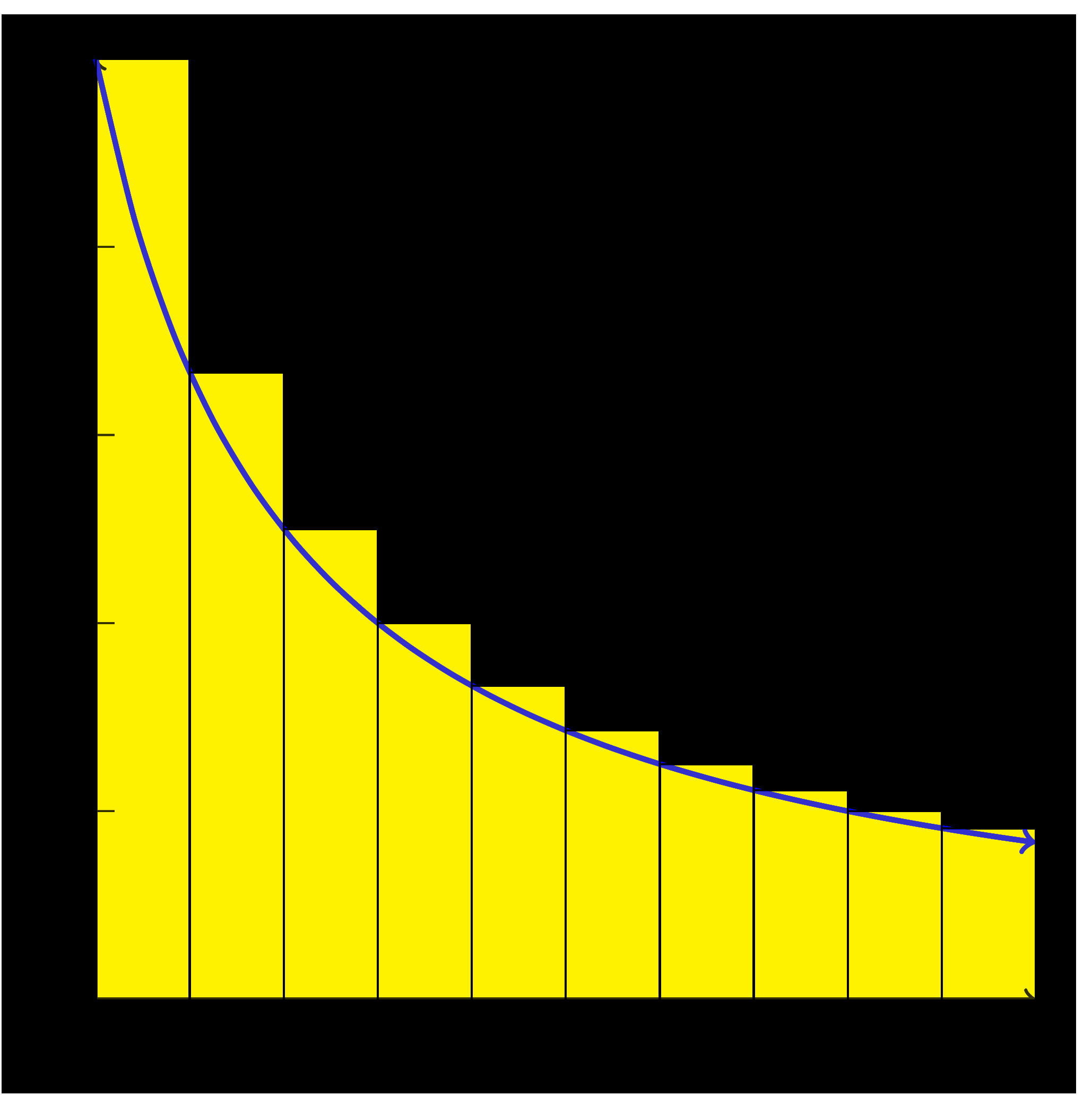
At this point we have used rectangles to estimate the total area underneath a curve. We will now explore a couple of different ways of constructing these rectangles. Consider the figures below. In Figure5.26 the rectangles are formed by setting the height of the rectangle so that the left side of the rectangle touches the curve. Conversely, in Figure5.27 the right side of the rectangle touches the curve. These are commonly called left hand approximations and right hand approximations respectively.
Figure5.26Left hand sum approximate to the area under the graph of the equation \(y=x\text{.}\)Figure5.27Right hand sum approximate to the area under the graph of the equation \(y=x\text{.}\)
In Figure5.26 you might notice that the left-hand approximation gives an underestimate for the total area of the curve. You might wonder what characteristics of a curve would ensure that a left-hand approximation is always underestimating the total area under the curve. You could similarly note that in Figure5.27 the right hand approximation gives an overestimate for the total area under the curve. Again, you might wonder what characteristics of a curve ensure this behavior.
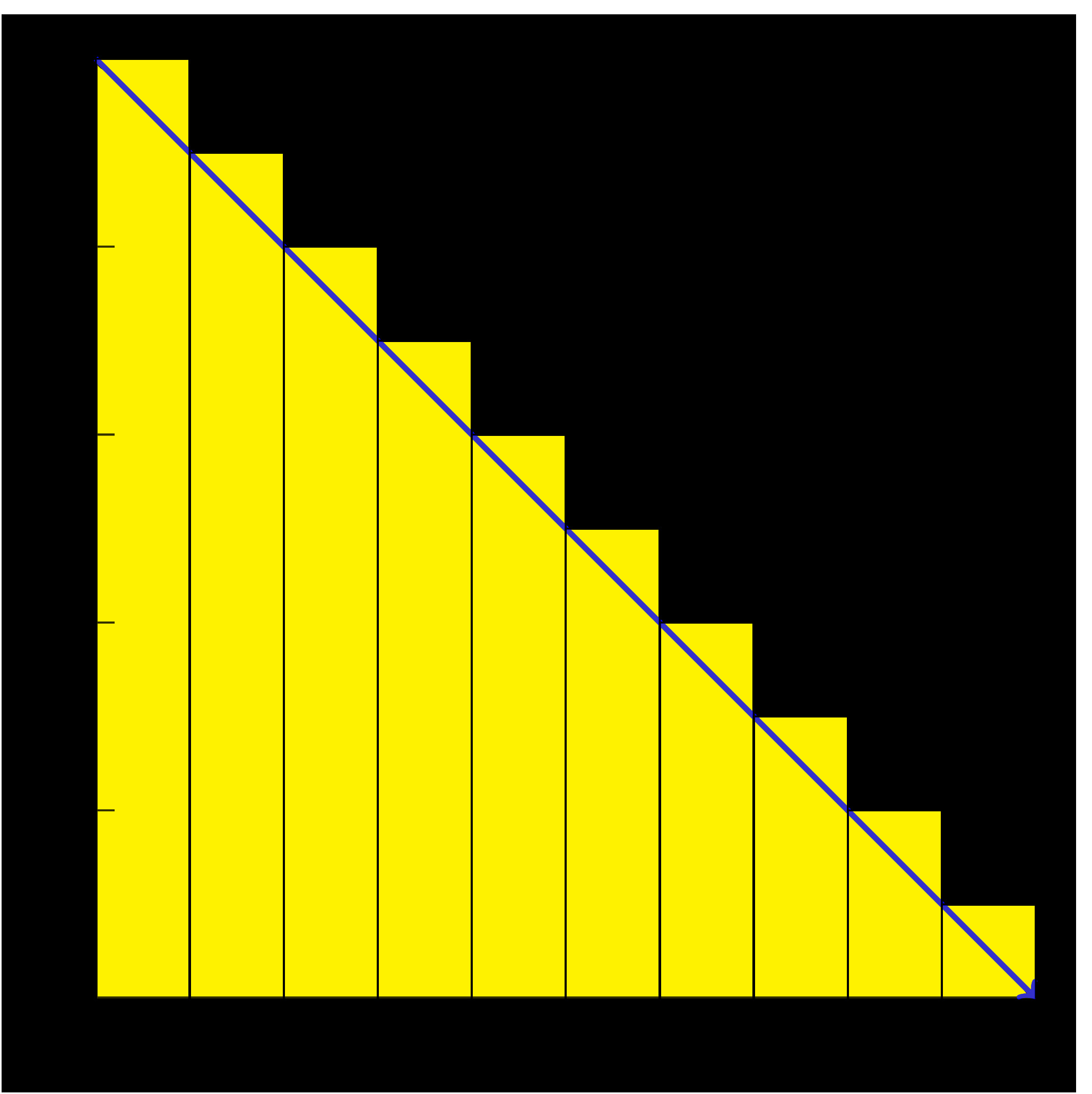
Figure5.28Various examples of left and right hand approximations.
Inspection of Figure5.28 might lead you to conclude that a left hand estimate is always an underestimate for an increasing function and an overestimate for a decreasing function, and that a right hand estimate is an overestimate for an increasing function and an underestimate for a decreasing function. This is indeed the case.
When approximating the area under a curve the following properties hold:
A left-hand estimate will overestimate the area under any portion of the curve on which it is decreasing.
A right-hand estimate will underestimate the area under any portion of the curve on which it is decreasing.
A left-hand estimate will underestimate the area under any portion of the curve on which it is increasing.
A right-hand estimate will overestimate the area under any portion of the curve on which it is decreasing.
Example5.29
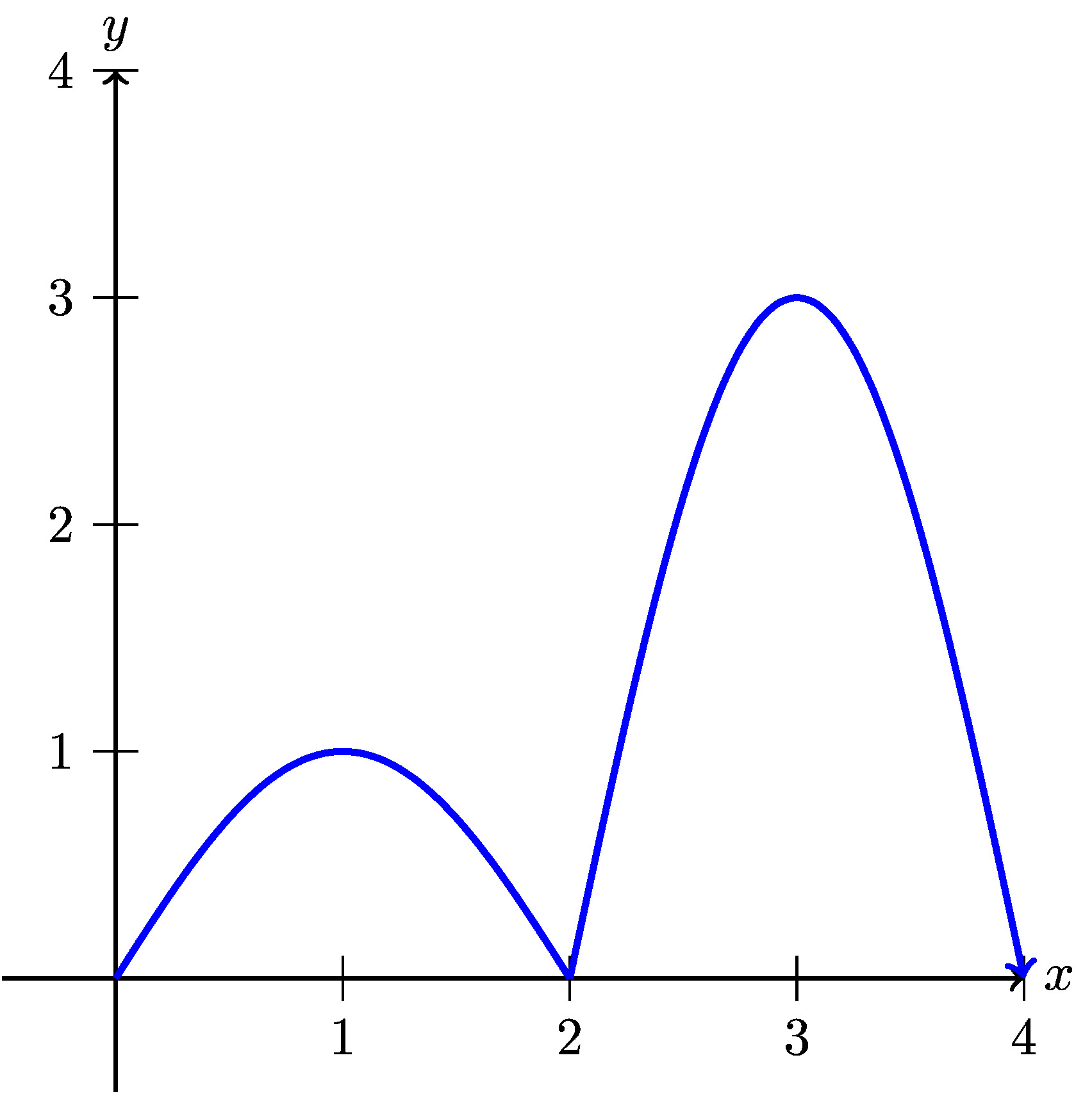
Consider the function whose graph is given in Figure5.30.
On what intervals is a left-hand estimate of the area an overestimate?
On what intervals is a right-hand estimate of the area an underestimate?
On what intervals is a left-hand estimate of the area an underestimate?
On what intervals is a right-hand estimate of the area an overestimate?
Figure5.30A function that is increasing and decreasing on various intervals..
A left-hand estimate will overestimate the area under any portion of the curve on which it is decreasing. Therefore, by inspecting Figure5.30 we can see that the figure is decreasing on \((1,2) \cup (3,4)\text{.}\) Note, we can also observe the overestimate in Figure5.31.
A right-hand estimate will underestimate the area under any portion of the curve on which it is decreasing. Therefore, by inspecting Figure5.30 we can see that the figure is decreasing on \((1,2) \cup (3,4)\text{.}\) Note, we can also observe the underestimate in Figure5.32.
A left-hand estimate will underestimate the area under any portion of the curve on which it is increasing. Therefore, by inspecting Figure5.30 we can see that the figure is increasing on \((0,1) \cup (2,3)\text{.}\) Note, we can also observe the underestimate in Figure5.31.
A right-hand estimate will overestimate the area under any portion of the curve on which it is increasing. Therefore, by inspecting Figure5.30 we can see that the figure is increasing on \((0,1) \cup (2,3)\text{.}\) Note, we can also observe the overestimate in Figure5.32.
Figure5.31Left hand sum approximate to the area under the graph from Figure5.30.Figure5.32Right hand sum approximate to the area under the graph from Figure5.30.
Subsection
Example5.33
A person walking along a straight path has her velocity in miles per hour at time \(t\) given by the function \(v(t) = 0.25t^3-1.5t^2+3t+0.25\text{,}\) for times in the interval \(0 \le t \le 2\text{.}\) The graph of this function is also given in each of the three diagrams in Figure5.34.
Figure5.34Three approaches to estimating the area under \(y = v(t)\) on the interval \([0,2]\text{.}\)
Note that in each diagram, we use four rectangles to estimate the area under \(y = v(t)\) on the interval \([0,2]\text{,}\) but the method by which the four rectangles' respective heights are decided varies among the three individual graphs.
How are the heights of rectangles in the left-most diagram being chosen? Explain, and hence determine the value of
Of the estimates \(S\text{,}\) \(T\text{,}\) and \(U\text{,}\) which do you think is the best approximation of \(D\text{,}\) the total distance the person traveled on \([0,2]\text{?}\) Why?
The heights of the rectangles are chosen by evaluating the function \(v(t) = 0.25t^3-1.5t^2+3t+0.25\) at the points in-between the right-hand and left-hand endpoints i.e. the midpoint. Specifically,
Visual inspection of the graphs makes it look like that \(U\) is the best approximation. The estimate \(S\) is clearly an under-estimate based on the graph; this can be further justified by the computation done in part (a). The estimate \(T\) is clearly an over-estimate based on the graph; this can be further justified by the computation done in part (b). Hence, the estimate \(U\) is a fairly accurate approximation.
SubsectionSigma Notation
We have used sums of areas of rectangles to approximate the area under a curve. Intuitively, we expect that using a larger number of thinner rectangles will provide a better estimate for the area. Consequently, we anticipate dealing with sums of a large number of terms. To do so, we introduce sigma notation, named for the Greek letter \(\Sigma\text{,}\) which is the capital letter \(S\) in the Greek alphabet.
We read the symbol \(\sum_{k=1}^{100} k\) as the sum from \(k\) equals 1 to 100 of \(k\text{.}\) The variable \(k\) is called the index of summation, and any letter can be used for this variable. The pattern in the terms of the sum is denoted by a function of the index; for example,
Sigma notation allows us to vary easily the function being used to describe the terms in the sum, and to adjust the number of terms in the sum simply by changing the value of \(n\text{.}\) We test our understanding of this new notation in the following example.
Example5.35
For each sum written in sigma notation, write the sum long-hand and evaluate the sum to find its value. For each sum written in expanded form, write the sum in sigma notation.
differs from the previous term by 4. If we view \(4\) as \(4 = 4 \cdot 1 - 1\) and \(7\) as \(7 = 4 \cdot 2 - 1\text{,}\) we see that the pattern may be represented through the function \(f(k) = 4k-1\text{,}\) so that
When a moving body has a positive velocity function \(y = v(t)\) on a given interval \([a,b]\text{,}\) the area under the curve over the interval gives the total distance the body travels on \([a,b]\text{.}\) We are also interested in finding the exact area bounded by \(y = f(x)\) on an interval \([a,b]\text{,}\) regardless of the meaning or context of the function \(f\text{.}\) For now, we continue to focus on finding an accurate estimate of this area by using a sum of the areas of rectangles. Unless otherwise indicated, we assume that \(f\) is continuous and non-negative on \([a,b]\text{.}\)
The first choice we make in such an approximation is the number of rectangles.
Figure5.36Subdividing the interval \([a,b]\) into \(n\) subintervals of equal length \(\Delta x\text{.}\)
If we desire \(n\) rectangles of equal width to subdivide the interval \([a,b]\text{,}\) then each rectangle must have width \(\Delta x = \frac{b-a}{n}\text{.}\) We let \(x_0 = a\text{,}\) \(x_n = b\text{,}\) and define \(x_{i} = a + i\Delta x\text{,}\) so that \(x_1 = x_0 + \Delta x\text{,}\) \(x_2 = x_0 + 2 \Delta x\text{,}\) and so on, as pictured in Figure5.36.
We use each subinterval \([x_i, x_{i+1}]\) as the base of a rectangle, and next choose the height of the rectangle on that subinterval. There are three standard choices: we can use the left endpoint of each subinterval, the right endpoint of each subinterval, or the midpoint of each. These are precisely the options encountered in Example5.33 and seen in Figure5.34. We next explore how these choices can be described in sigma notation.
Consider an arbitrary positive function \(f\) on \([a,b]\) with the interval subdivided as shown in Figure5.36, and choose to use left endpoints. Then on each interval \([x_{i}, x_{i+1}]\text{,}\) the area of the rectangle formed is given by
Figure5.37Subdividing the interval \([a,b]\) into \(n\) subintervals of equal length \(\Delta x\) and approximating the area under \(y = f(x)\) over \([a,b]\) using left rectangles.
If we let \(L_n\) denote the sum of the areas of these rectangles, we see that
Note that since the index of summation begins at \(0\) and ends at \(n-1\text{,}\) there are indeed \(n\) terms in this sum. We call \(L_n\) the left Riemann sum for the function \(f\) on the interval \([a,b]\text{.}\)
To see how the Riemann sums for right endpoints and midpoints are constructed, we consider Figure5.38.
Figure5.38Riemann sums using right endpoints and midpoints.
For the sum with right endpoints, we see that the area of the rectangle on an arbitrary interval \([x_i, x_{i+1}]\) is given by \(B_{i+1} = f(x_{i+1}) \cdot \Delta x\text{,}\) and that the sum of all such areas of rectangles is given by
so that \(\overline{x}_{i+1}\) is the midpoint of the interval \([x_i, x_{i+1}]\text{.}\) For instance, for the rectangle with area \(C_1\) in Figure5.38, we now have
and we say that \(M_n\) is the middle Riemann sum for \(f\) on \([a,b]\text{.}\)
Thus, we have two variables to explore: the number of rectangles and the height of each rectangle. We can explore these choices dynamically, and the applet3Marc Renault, Geogebra Calculus Applets. found at http://gvsu.edu/s/a9 is a particularly useful one. There we see the image shown in Figure5.39, but with the opportunity to adjust the slider bars for the heights and the number of rectangles.
By moving the sliders, we can see how the heights of the rectangles change as we consider left endpoints, midpoints, and right endpoints, as well as the impact that a larger number of narrower rectangles has on the approximation of the exact area bounded by the function and the horizontal axis.
When \(f(x) \ge 0\) on \([a,b]\text{,}\) each of the Riemann sums \(L_n\text{,}\) \(R_n\text{,}\) and \(M_n\) provides an estimate of the area under the curve \(y = f(x)\) over the interval \([a,b]\text{.}\) We also recall that in the context of a nonnegative velocity function \(y = v(t)\text{,}\) the corresponding Riemann sums approximate the distance traveled on \([a,b]\) by a moving object with velocity function \(v\text{.}\)
There is a more general way to think of Riemann sums, and that is to allow any choice of where the function is evaluated to determine the rectangle heights. Rather than saying we'll always choose left endpoints, or always choose midpoints, we simply say that a point \(x_{i+1}^*\) will be selected at random in the interval \([x_i, x_{i+1}]\) (so that \(x_i \le x_{i+1}^* \le x_{i+1}\)). The Riemann sum is then given by
\begin{equation*}
f(x_1^*) \cdot \Delta x + f(x_2^*) \cdot \Delta x + \cdots + f(x_{i+1}^*) \cdot \Delta x + \cdots + f(x_n^*) \cdot \Delta x = \sum_{i=1}^{n} f(x_i^*) \Delta x\text{.}
\end{equation*}
At http://gvsu.edu/s/a9, the applet noted earlier and referenced in Figure5.39, by unchecking the relative box at the top left, and instead checking random, we can easily explore the effect of using random point locations in subintervals on a Riemann sum. In computational practice, we most often use \(L_n\text{,}\) \(R_n\text{,}\) or \(M_n\text{,}\) while the random Riemann sum is useful in theoretical discussions. In the following example, we investigate several different Riemann sums for a particular velocity function.
Example5.40
Suppose that an object moving along a straight line path has its velocity in feet per second at time \(t\) in seconds given by \(v(t) = \frac{2}{9}(t-3)^2 + 2\text{.}\)
Carefully sketch the region whose exact area will tell you the value of the distance the object traveled on the time interval \(2 \le t \le 5\text{.}\)
Estimate the distance traveled on \([2,5]\) by computing \(L_4\text{,}\) \(R_4\text{,}\) and \(M_4\text{.}\)
Does averaging \(L_4\) and \(R_4\) result in the same value as \(M_4\text{?}\) If not, what do you think the average of \(L_4\) and \(R_4\) measures?
For this question, think about an arbitrary function \(f\text{,}\) rather than the particular function \(v\) given above. If \(f\) is positive and increasing on \([a,b]\text{,}\) will \(L_n\) over-estimate or under-estimate the exact area under \(f\) on \([a,b]\text{?}\) Will \(R_n\) over- or under-estimate the exact area under \(f\) on \([a,b]\text{?}\) Explain.
This average actually measures what would result from using four trapezoids, rather than rectangles, to estimate the area on each subinterval. One reason this is so is because the area of a trapezoid is the average of the bases times the width, and the bases are given by the function values at the left and right endpoints.
If \(f\) is positive and increasing on \([a,b]\text{,}\) \(L_n\) will under-estimate the exact area under \(f\) on \([a,b]\text{.}\) Because \(f\) is increasing, its value at the left endpoint of any subinterval will be lower than every other function value in the interval, and thus the rectangle with that height lies exclusively below the curve. In a similar way, \(R_n\) over-estimates the exact area under \(f\) on \([a,b]\text{.}\)
we can of course compute the sum even when \(f\) takes on negative values. We know that when \(f\) is positive on \([a,b]\text{,}\) a Riemann sum estimates the area bounded between \(f\) and the horizontal axis over the interval.
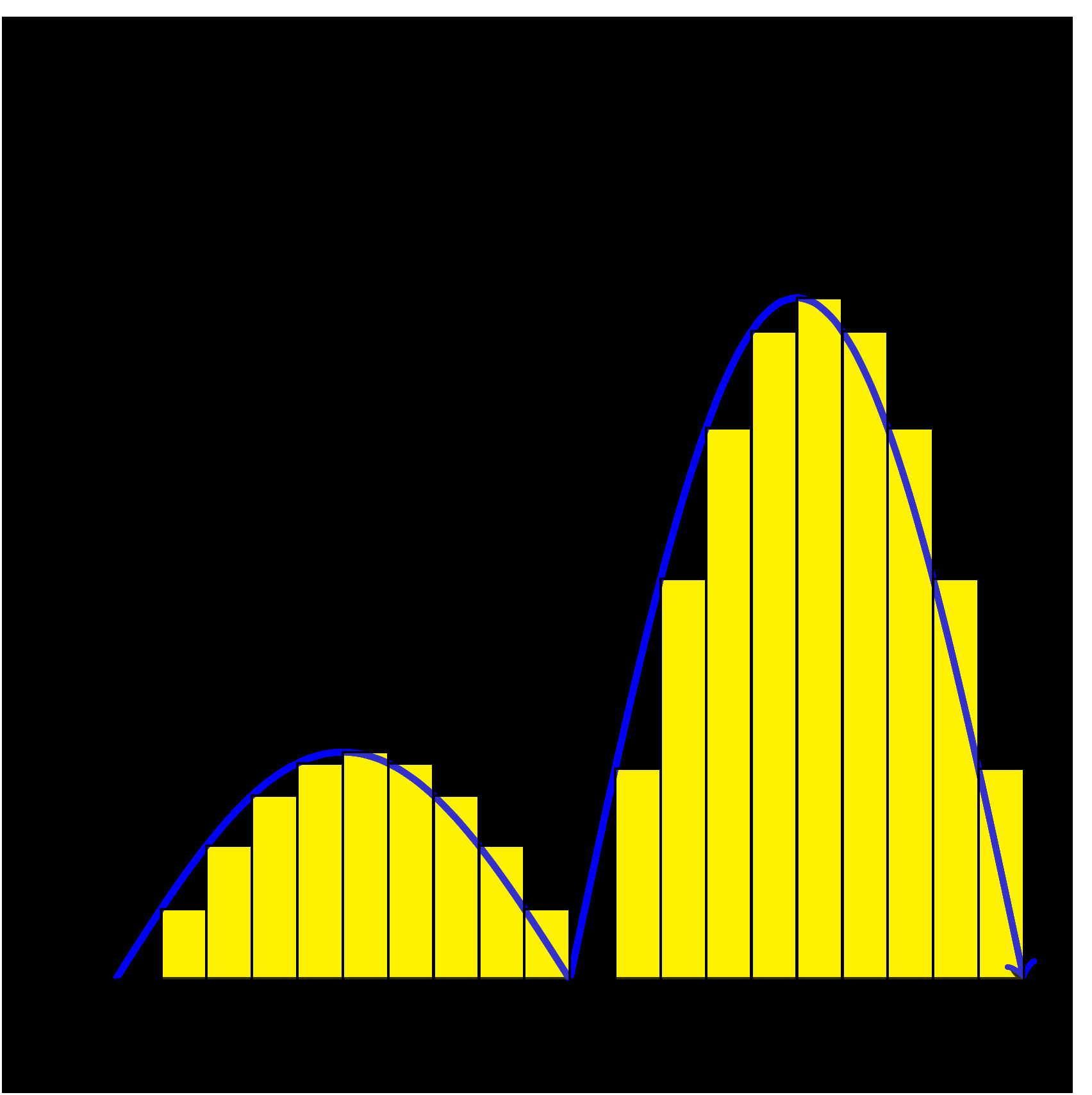
Figure5.41At left and center, two left Riemann sums for a function \(f\) that is sometimes negative; at right, the areas bounded by \(f\) on the interval \([a,d]\text{.}\)
For the function pictured in the first graph of Figure5.41, a left Riemann sum with 12 subintervals over \([a,d]\) is shown. The function is negative on the interval \(b \le x \le c\text{,}\) so at the four left endpoints that fall in \([b,c]\text{,}\) the terms \(f(x_i) \Delta x\) are negative. This means that those four terms in the Riemann sum produce an estimate of the opposite of the area bounded by \(y = f(x)\) and the \(x\)-axis on \([b,c]\text{.}\)
In the middle graph of Figure5.41, we see that by increasing the number of rectangles the approximation of the area (or the opposite of the area) bounded by the curve appears to improve.
In general, any Riemann sum of a continuous function \(f\) on an interval \([a,b]\) approximates the difference between the area that lies above the horizontal axis on \([a,b]\) and under \(f\) and the area that lies below the horizontal axis on \([a,b]\) and above \(f\text{.}\) In the notation of Figure5.41, we may say that
where \(L_{24}\) is the left Riemann sum using 24 subintervals shown in the middle graph. \(A_1\) and \(A_3\) are the areas of the regions where \(f\) is positive, and \(A_2\) is the area where \(f\) is negative. We will call the quantity \(A_1 - A_2 + A_3\) the net signed area bounded by \(f\) over the interval \([a,d]\text{,}\) where by the phrase signed area we indicate that we are attaching a minus sign to the areas of regions that fall below the horizontal axis.
Finally, we recall that if the function \(f\) represents the velocity of a moving object, the sum of the areas bounded by the curve tells us the total distance traveled over the relevant time interval, while the net signed area bounded by the curve computes the object's change in position on the interval.
Example5.42
Suppose that an object moving along a straight line path has its velocity \(v\) (in feet per second) at time \(t\) (in seconds) given by
Compute \(M_5\text{,}\) the middle Riemann sum, for \(v\) on the time interval \([1,5]\text{.}\) Be sure to clearly identify the value of \(\Delta t\) as well as the locations of \(t_0\text{,}\) \(t_1\text{,}\) \(\cdots\text{,}\) \(t_5\text{.}\) In addition, provide a careful sketch of the function and the corresponding rectangles that are being used in the sum.
Building on your work in (a), estimate the total change in position of the object on the interval \([1,5]\text{.}\)
Building on your work in (a) and (b), estimate the total distance traveled by the object on \([1,5]\text{.}\)
Use appropriate computing technology4For instance, consider the applet at http://gvsu.edu/s/a9 and change the function and adjust the locations of the blue points that represent the interval endpoints \(a\) and \(b\text{.}\) to compute \(M_{10}\) and \(M_{20}\text{.}\) What exact value do you think the middle sum eventually approaches as \(n\) increases without bound? What does that number represent in the physical context of the overall problem?
For this Riemann sum with five subintervals, \(\Delta t = \frac{5-1}{5} = \frac{4}{5}\text{,}\) so \(t_0 = 1\text{,}\) \(t_1 = 1.8\text{,}\) \(t_2 = 2.6\text{,}\) \(t_3 = 3.4\text{,}\) \(t_4 = 4.2\) and \(t_5 = 4\text{.}\) It follows that
Since the net signed area bounded by \(v\) on \([1,5]\) represents the total change in position of the object on the interval \([1,5]\text{,}\) it follows that \(M_5\) estimates the total change in position. Hence, the change in position is approximately \(-1.44\) feet.
To estimate the total distance traveled by the object on \([1,5]\text{,}\) we have to calculate the total area between the curve and the \(t\)-axis. Thus,
Using appropriate technology, \(M_{10} = -1.36\) and \(M_{20} = -1.34\text{.}\) Further calculations suggest that \(M_n \to -\frac{4}{3} = -1.\overline{33}\) as \(n \to \infty\text{,}\) and this number represents the object's total change in position on \([1,5]\text{.}\)
SubsectionThe Definition of the Definite Integral
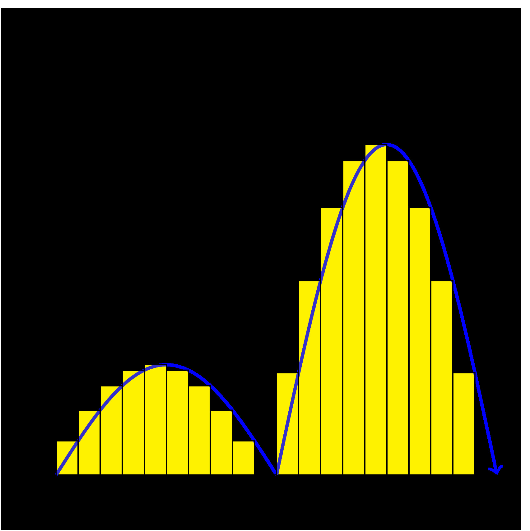
In Figure5.43, we see evidence that increasing the number of rectangles in a Riemann sum improves the accuracy of the approximation of the net signed area bounded by the given function.
Figure5.43At left and center, two left Riemann sums for a function \(f\) that is sometimes negative; at right, the exact areas bounded by \(f\) on the interval \([a,d]\text{.}\)
We therefore explore the natural idea of allowing the number of rectangles to increase without bound. In an effort to compute the exact net signed area we also consider the differences among left, right, and middle Riemann sums and the different results they generate as the value of \(n\) increases. We begin with functions that are exclusively positive on the interval under consideration.
In Figure5.43, we saw that as the number of rectangles got larger and larger, the values of \(L_n\) converge to some value. It turns out that any continuous function on an interval \([a,b]\text{,}\) \(L_n\) and \(R_n\) will converge to the same value as \(n\) grows larger. In fact, for any continuous function and a Riemann sum using any point \(x_{i+1}^*\) in the interval \([x_i, x_{i+1}]\text{,}\) \(\lim_{n \to \infty} \sum_{i=1}^{n} f(x_i^*) \Delta x\) will converge to that same value. Thus, as we let \(n \to \infty\text{,}\) it doesn't really matter where we choose to evaluate the function within a given subinterval, because
The fact that these limits always exist (and share the same value) when \(f\) is continuous5It turns out that a function need not be continuous in order to have a definite integral. For our purposes, we assume that the functions we consider are continuous on the interval(s) of interest. It is straightforward to see that any function that is piecewise continuous on an interval of interest will also have a well-defined definite integral. allows us to make the following definition.
The definite integral of a continuous function \(f\) on the interval \([a,b]\text{,}\) denoted \(\int_a^b f(x) \, dx\text{,}\) is the real number given by
where \(\Delta x = \frac{b-a}{n}\text{,}\) \(x_i = a + i\Delta x\) (for \(i = 0, \ldots, n\)), and \(x_i^*\) satisfies \(x_{i-1} \le x_i^* \le x_i\) (for \(i = 1, \ldots, n\)).
We call the symbol \(\int\) the integral sign, the values \(a\) and \(b\) the limits of integration, and the function \(f\) the integrand The process of determining the real number \(\int_a^b f(x) \, dx\) is called evaluating the definite integral. While there are several different interpretations of the definite integral, for now the most important is that \(\int_a^b f(x) \, dx\) measures the net signed area bounded by \(y = f(x)\) and the \(x\)-axis on the interval \([a,b]\text{.}\)
For example, if \(f\) is the function pictured in Figure5.44, and \(A_1\text{,}\) \(A_2\text{,}\) and \(A_3\) are the exact areas bounded by \(f\) and the \(x\)-axis on the respective intervals \([a,b]\text{,}\) \([b,c]\text{,}\) and \([c,d]\text{,}\) then
Figure5.44A continuous function \(f\) on the interval \([a,d]\text{.}\)
We can also use definite integrals to express the change in position and the distance traveled by a moving object. If \(v\) is a velocity function on an interval \([a,b]\text{,}\) then the change in position of the object, \(s(b) - s(a)\text{,}\) is given by
If the velocity function is nonnegative on \([a,b]\text{,}\) then \(\int_a^b v(t) \,dt\) tells us the distance the object traveled. If the velocity is sometimes negative on \([a,b]\text{,}\) we can use definite integrals to find the areas bounded by the function on each interval where \(v\) does not change sign, and the sum of these areas will tell us the distance the object traveled.
To compute the value of a definite integral from the definition, we have to take the limit of a sum. While this is possible to do in select circumstances, it is also tedious and time-consuming.
SubsectionSummary
If we know the velocity of a moving object at every point in a given interval, then we can determine the distance the object has traveled on that time interval by finding the area under the velocity function on that interval. We can also determine the position of the object by taking into account that the position function is decreasing when the velocity is negative.
When we cannot compute the area under the velocity curve exactly, we can use rectangles to estimate the area. The heights of the rectangles are determined by the values of the velocity function, and we must make a choice of what values we use, such as the left endpoint, the right endpoint, the midpoint, etc. We then find the sum of the areas of the rectangles, called a Riemann sum, and this is our estimate for the net signed area under the curve.
Often we will use sigma notation when writing out the sum that we obtain from adding up the areas of the rectangles. For example, if we want to compute \(L_n \text{,}\) then using sigma notation we can write \(L_n = \sum_{i = 0}^{n-1} f(x_i) \Delta x
\text{,}\) where \(x_i \) is the left endpoint of the \(i+1 \) rectangle, as seen in Figure5.37.
The more rectangles we use, the more accurate our estimate will be. In fact, if we continue to increase the number of intervals and take the limit of these estimates, we obtain the exact area, called the definite integral. Notationally, this is given by
Suppose that the velocity of a moving object is given by \(v(t) = t(t-1)(t-3)\text{,}\) measured in feet per second, and that this function is valid for \(0 \le t \le 4\text{.}\)
Write an expression involving definite integrals whose value is the total change in position of the object on the interval \([0,4]\text{.}\)
Use appropriate technology (such as http://gvsu.edu/s/a96Marc Renault, Shippensburg University.) to compute Riemann sums to estimate the object's total change in position on \([0,4]\text{.}\) Work to ensure that your estimate is accurate to two decimal places, and explain how you know this to be the case.
Write an expression involving definite integrals whose value is the total distance traveled by the object on \([0,4]\text{.}\)
Use appropriate technology to compute Riemann sums to estimate the object's total distance travelled on \([0,4]\text{.}\) Work to ensure that your estimate is accurate to two decimal places, and explain how you know this to be the case.
What is the object's average velocity on \([0,4]\text{,}\) accurate to two decimal places?
The velocity of an object moving along an axis is given by the piecewise linear function \(v\) that is pictured in Figure5.45. Assume that the object is moving to the right when its velocity is positive, and moving to the left when its velocity is negative. Assume that the given velocity function is valid for \(t = 0\) to \(t = 4\text{.}\)
Write an expression involving definite integrals whose value is the total change in position of the object on the interval \([0,4]\text{.}\)
Use the provided graph of \(v\) to determine the value of the total change in position on \([0,4]\text{.}\)
Write an expression involving definite integrals whose value is the total distance traveled by the object on \([0,4]\text{.}\) What is the exact value of the total distance traveled on \([0,4]\text{?}\)
What is the object's exact average velocity on \([0,4]\text{?}\)
Find an algebraic formula for the object's position function on \([0, 1.5]\) that satisfies \(s(0) = 0\text{.}\)
Figure5.45The velocity function of a moving object.