Kevin Gonzales, Eric Hopkins, Catherine Zimmitti, Cheryl Kane, Modified to fit Applied Calculus from Coordinated Calculus by Nathan Wakefield et. al., Based upon Active Calculus by Matthew Boelkins
Section4.5Tangent Line Approximations
Motivating Questions
For a general differentiable function, how can we use the derivative of a function to approximate the values of the function?
What is the marginal Profit, Revenue, and Cost? How can we use these to approximate the Profit, Revenue, and Cost functions?
Often in business, explicit formulas for Cost, Revenue, and Profit (\(C(x)\text{,}\) \(R(x)\text{,}\) and \(P(x)\) respectively) are not known. However, information may exist about the cost, revenue and profit trends at a particular value \(x=a\text{.}\) For example, suppose that you are running a company that produces and sells computers. In an ideal world, you would have a function, \(P(x)\text{,}\) for the profit from the sale of \(x\) computers. However, in the real world, you only know that the profit from the sale of 100 laptops is \(P(100)=\$5000\text{.}\) You also know that the profit increased by \(\$100\) per laptop when 100 laptops are sold.
From this information you could make an estimate that the profit from the sale of 101 computers would be \(P(101)\approx 5100\text{.}\) It is important to note that you can not assume that the profit grows at a linear (i.e. constant) rate! There are many variables when producing and selling an item, and for many companies a profit is not made unless a certain number of units are sold.
Without creating an explicit function for the profit, can we estimate future profits? In this section, we will explore how to use the derivative (or rate of change) of a function to estimate the values of the function.
SubsectionLinear Approximations
Among all functions, linear functions are simplest. One of the powerful consequences of a function \(y = f(x)\) being differentiable at a point \((a,f(a))\) is that up close the function \(y = f(x)\) is locally linear and looks like its tangent line at that point. In certain circumstances, this allows us to approximate the original function \(f\) with a simpler function \(L\) that is linear: this can be advantageous when we have limited information about \(f\) or when \(f\) is computationally or algebraically complicated. We will explore all of these situations in what follows.
It is essential to recall that when \(f\) is differentiable at \(x = a\text{,}\) the value of \(f'(a)\) provides the slope of the tangent line to \(y = f(x)\) at the point \((a,f(a))\text{.}\) If we know both a point on the tangent line and the slope of the line we can find the equation of the tangent line and write the equation in point-slope form.8Recall that a line with slope \(m\) that passes through \((x_0,y_0)\) has equation \(y - y_0 = m(x - x_0)\text{,}\) and this is the point-slope form of the equation.
Example4.51
Consider the function \(g(x) = -x^2+3x+2\text{.}\)
Find the derivative \(g'(x)\text{.}\)
Determine the slope of the tangent line to the graph of \(y = g(x)\) at the value \(x = 2\text{.}\)
Compute \(g(2)\text{.}\)
Find an equation for the tangent line to the graph of \(y = g(x)\) at the point \((2,g(2))\text{.}\) Write your result in point-slope form.
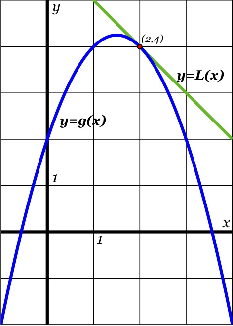
Sketch an accurate, labeled graph of \(y = g(x)\) on the interval \(-1\le x\le4\text{.}\) On the same axes, sketch its tangent line at the point \((2,g(2))\text{.}\)
Figure4.53The graph of \(y=g(x)\) along with its tangent line \(L\) at the point \((2,4)\text{,}\) where \(g(x)=-x^2+3x+2\text{.}\)
SubsectionThe Tangent Line
Given a function \(f\) that is differentiable at \(x = a\text{,}\) we know that we can determine the slope of the tangent line to \(y = f(x)\) at \((a,f(a))\) by computing \(f'(a)\text{.}\) This allows us to write the equation for the tangent line as follows:
The Tangent Line
The equation of the resulting tangent line is given in point-slope form by
\begin{equation*}
y - f(a) = f'(a)(x-a) \text{.}
\end{equation*}
Warning4.54
Note: there is a major difference between \(f(a) \) and \(f(x) \) in this context. The former is a constant that results from using the given fixed value of \(a\text{,}\) while the latter is the general expression for the rule that defines the function. The same is true for \(f'(a)\) and \(f'(x)\text{:}\) we must carefully distinguish between these expressions. Each time we find the tangent line, we need to evaluate the function and its derivative at a fixed \(a\)-value.
In Figure4.55 below, we see the graph of a function \(f\) and its tangent line at the point \((a,f(a))\text{.}\) Notice how when we zoom in we see the local linearity of \(f\) more clearly highlighted. The function and its tangent line are nearly indistinguishable up close. Local linearity can also be seen dynamically in the java applet at http://gvsu.edu/s/6J.
Figure4.55The graph of a function \(y = f(x)\) and its tangent line at the point \((a,f(a))\text{:}\) at left, from a distance, and at right, up close. If we let \(L(x)=f'(a)(x-a)+f(a)\) denote the tangent line function, then we observe in the right image that for \(x\) near \(a\text{,}\) \(f(x) \approx L(x)\text{.}\)
SubsectionApproximations
A slight change in perspective and notation will enable us to be more precise in discussing how the tangent line approximates \(f(x)\) near \(x = a\text{.}\) By solving for \(y\text{,}\) we can write the equation for the tangent line as
\begin{equation*}
y = f'(a)(x-a) + f(a)\text{.}
\end{equation*}
This line is itself a function of \(x\text{.}\) Replacing the variable \(y\) with the expression \(L(x)\text{,}\) we have the following.
the tangent line approximation of \(f\) at the point \((a,f(a))\).
In this notation, \(L(x)\) is nothing more than a "new name" for the tangent line. As we saw above, for \(x\) close to \(a\text{,}\) \(f(x) \approx L(x)\text{.}\)
Example4.56Using the Tangent Line Approximation
Suppose that it is known that, for a given differentiable function \(y = f(x)\text{,}\) its tangent line approximation at the point \(x = 1 \) is given by
Note that we may reason through part b) in a different way as well. We know that the tangent line approximation \(L(x)\) to a function at a point \((a,f(a))\) "touches" the function at that point, so \(L(a)\) must be the same as \(f(a)\text{.}\) In this case, since the tangent line was was approximated at the point \(a=1\text{,}\) we know that \(f(1)=L(1)=3\text{.}\) Further, we know that the (constant) slope of the tangent line approximation was defined to be the slope of \(f\) at \(x=a\text{.}\) We could rewrite \(L(x)\) in slope-intercept form as \(-2x+5\) and see that its slope is \(-2\) (or we could take the derivative of \(L(x)\) to find that \(L'(x)=-2\)). In either case, we see that the \(f'(1)\) equals \(-2\text{,}\) the slope of the tangent line approximation.
Example4.57Error in a Tangent Line Approximation
Consider the function \(p(t)=\ln(t)\text{.}\)
Find the tangent line approximation, \(L(t)\text{,}\) of \(p\) at \(t=1\text{.}\)
Use the tangent line approximation from (a) to estimate the value of \(\ln(1.01)\text{.}\)
Use the tangent line approximation from (a) to estimate the value of \(\ln(1.3)\text{.}\)
The error of an approximation is the difference between the true value and the estimated value. In particular, given a function \(f\) and its tangent line approximation \(L(x)\) at \((a,f(a))\text{,}\) we say the error of the tangent line approximation is
Of the two estimates you found in (b) and (c), which do you expect to be more accurate? Why? Check your guess by calculating and comparing \(E(1.01)\) and \(E(1.3)\text{.}\)
We start by computing \(p'(t)\text{,}\) and then evaluating \(p(1)\) and \(p'(1)\text{.}\) Since \(p(t)=\ln(t)\text{,}\) the derivative is \(p'(t)=\frac1t\text{.}\) Furthermore, we have \(p(1)=\ln(1)=0\) and \(p'(1)=\frac11=1\text{.}\) Thus, the tangent line approximation of \(p(t)=\ln(t)\) at the point \((1,0)\) is
Since we can use the tangent line approximation for \(p\) at \((1,0)\) to estimate output values of \(p\) at nearby points, it follows that \(p(1.01)\approx L(1.01)\text{.}\) Thus we have
Since we can use the tangent line approximation for \(p\) at \((1,0)\) to estimate output values of \(p\) at nearby points, it follows that \(p(1.3)\approx L(1.3)\text{.}\) Thus we have
Since \(1.3\) is farther away from the point of tangency \((t=1)\) than \(1.01\) is, we expect the estimate to be better for \(1.01\text{.}\) We confirm this by computing the error at each point, finding that
As expected, the error grew as the point moved farther from the initial point of tangency.
We emphasize that \(L(x)\) is simply a new name for the tangent line function. Using this new notation and our observation that \(L(x) \approx f(x)\) for \(x\) near \(a\text{,}\) it follows that we can write
We now seek to apply approximation techniques to specific business concepts.
Suppose we have a cost function \(C(n)\text{,}\) giving information about the cost of selling \(n\) items. Building a tangent line approximation at \(a=x\text{,}\) we know from (4.1) that
\begin{equation*}
C(n) \approx C(x) + C'(x) (n-x) \ \text{for} \ n \ \text{near} \ x
\end{equation*}
Notice from the right-hand side that we only need to know information about the cost function for a specific number of items \(x\text{,}\) and we use this to approximate the cost function for a number of items \(n\) that is close to \(x\text{.}\) What about the next item sold, number \(x+1\text{?}\) For \(n=x+1\text{,}\) we would have
We will use the principle given by (4.2) a few times below with the Cost, Revenue, and Profit functions.
Marginal Cost, Revenue and Profit
The marginal cost is the derivative \(C'(x)\) of the cost function. If we know the cost of selling \(x \) items, then the marginal cost is used to approximate the cost of \(x+1\) items (by the reasoning used to obtain (4.2)) as follows:
The marginal revenue is the derivative \(R'(x)\) of the revenue function. If we know the revenue from selling \(x \) items, then the marginal revenue is used to approximate the revenue from selling \(x+1\) items (by the reasoning used to obtain (4.2)) as follows:
The marginal profit is the derivative \(P'(x)\) of the profit function. If we know the profit from selling \(x \) items, then the marginal profit is used to approximate the profit from selling \(x+1\) items (by the reasoning used to obtain (4.2)) as follows:
What is the current monthly cost? What is the current marginal cost?
What would be the additional cost of increasing the production to 26 backpacks monthly?
Using the marginal cost, what is the approximate cost to produce the 26th backpack monthly? Compare this to the actual additional cost computed in part (b).
Use the marginal cost to estimate \(C(27)\text{,}\) \(C(28)\text{,}\) and \(C(23)\text{.}\)
The approximate cost to produce the 26th item is \(C'(25)=24.38\text{,}\) the real cost is \(24.52\text{,}\) thus the approximation is only off by 14 cents!
The approximate cost to produce the 26th item is \(C'(25)=24.38\text{,}\) and the real cost is \(24.52\text{.}\) Thus the approximation is only off by 14 cents!
To estimate the cost of producing 27 backpacks we can use:
What is the current weekly profit? What is the current marginal profit?
How much profit would be lost if the dealership were able to sell only \(59\) cars weekly? How does this value compare to the marginal profit found in part (a)?
Use the marginal profit to estimate the weekly profit if the sales increase to \(61\) cars weekly, \(62\) cars weekly, and \(65\) cars weekly.
Approximate profit when \(61\) cars are sold weekly is \(\$51595.20\text{.}\) Approximate profit when \(62\) cars are sold weekly is \(\$52406.40\text{.}\) Approximate profit when \(61\) cars are sold weekly is \(\$54840\text{.}\)
Of course, the final part of these examples are just estimates. If we have an explicit function for \(C(x)\) and \(P(x)\) in the real world, then we would never use an estimate. However, often in the real world we only have the information at a point and not an explicit function. This example demonstrates how we could approximate.
Example4.60
Suppose that a company that sells widgets determines that the daily revenue, \(R(x),\) in dollars, from the sale of \(75\) widgets are sold is \(900\) dollars. The marginal revenue when \(75\) widgets are sold is \(11\) dollars per widget.
Estimate the daily revenue from the sale of \(77\) widgets.
Estimate the daily revenue from the sale of \(80\) widgets.
Estimate the daily revenue from the sale of \(74\) widgets.
Here we are not given the revenue function. However, we are given \(R(75)=900\) and \(R'(75)=11\text{.}\) In the real world these are values that could be computed even without ever finding an explicit revenue function. We can use this information to approximate the revenue from the sale of \(77\) items:
We start at \(75\) since this is the only information given, then we multiply the marginal revenue by \(2\) since we have sold \(2\) more widgets to get to a total of \(77\) widgets.
We start at \(75\) since this is the only information given, then we multiply the marginal revenue by \(5\) since we have sold \(5\) more widgets to get to a total of \(80\) widgets.
We start at \(75\) since this is the only information given, then we multiply the marginal revenue by \(-1\) since we have sold \(1\) less widgets to get to a total of \(74\) widgets.
SubsectionSummary
The tangent line to a differentiable function \(y = f(x)\) at the point \((a,f(a))\) is given in point-slope form by the equation
\begin{equation*}
y - f(a) = f'(a)(x-a)\text{.}
\end{equation*}
For a function \(f \) which is differentiable at \(x=a \text{,}\) we can use the equation for tangent line \(L(x) = f(a) + f'(a)(x-a)\) to approximate \(f \) near \(a \text{.}\) We often call \(L(x) \) the tangent line approximation of \(f \) at \(a \) (or you may see it referred to as the local linearization of \(f\) at \(a\)). Marginal cost, revenue, and profit are an example of using the tangent line approximation of the cost, revenue, and profit functions respectively to approximate these functions.
The marginal cost is the derivative \(C'(x) \) of the cost function, the marginal revenue is the derivative \(R'(x) \) of the revenue function, and the marginal profit is the derivative \(P'(x) \) of the profit function. If we know the cost of selling \(x \) items, then the marginal cost can be used to estimate the cost of selling another amount of items, if that amount is near \(x \text{.}\) The same holds true for the marginal revenue and marginal profit functions.