Kevin Gonzales, Eric Hopkins, Catherine Zimmitti, Cheryl Kane, Modified to fit Applied Calculus from Coordinated Calculus by Nathan Wakefield et. al., Based upon Active Calculus by Matthew Boelkins
Section1.1Introduction to Limits
Motivating Questions
What is the mathematical notion of limit and what role do limits play in the study of functions?
What is the meaning of the notation \(\displaystyle \lim_{x \to a} f(x) = L\text{?}\)
How do we go about determining the value of the limit of a function at a point?
What is a left-hand limit at \(x = a\) and a right-hand limit at \(x = a\text{?}\)
What does it mean graphically to say that \(f\) has limit \(L\) as \(x \to a\text{?}\) How is this connected to having a left-hand limit at \(x = a\) and having a right-hand limit at \(x=a\text{?}\)
Limits are a mathematical construct we can use to describe the behavior of a function near a point. Why might we want to consider the behavior near a point instead of at the point? Consider the function \(\displaystyle f(x)=\frac{x^2-25}{x-5}\text{.}\) The domain of \(f(x)\) is \(x\neq 5\text{,}\) that is the domain is all \(x\) not equal to \(5\text{.}\) Thus we can say that \(f(5)\) does not exists (DNE). Since we can not plug in \(x=5\text{,}\) we will instead seek to understand what happens to \(f(x)\) as \(x\) gets closer and closer, but not equal to, \(5\text{.}\) We can try to answer this question by simply plugging in values of \(x\) that are getting closer and closer to \(5\) into \(f(x)\text{,}\) see Table1.1.
\(x\)
\(\displaystyle f(x)=\frac{x^2-25}{x-5}\)
\(4.9\)
\(9.9\)
\(4.99\)
\(9.99\)
\(4.999\)
\(9.999\)
\(4.9999\)
\(9.9999\)
\(5.0001\)
\(10.0001\)
\(5.001\)
\(10.001\)
\(5.01\)
\(10.01\)
\(5.1\)
\(10.1\)
Table1.1Table of \(g\) values near \(x=5\text{.}\)
Observe that as \(x\) gets closer and closer, but not equal to \(5\text{,}\) the function values are getting closer and closer to \(10\text{.}\)
Instead of filling out a table of values, we could instead look at the graph of a function and ask the same question. What happens to the function as \(x\) gets closer and closer, but not equal to, a particular value? Consider the function \(g\) given by the graph in Figure1.2 below. We can evaluate the function at a variety of points. For example, \(g(-2)=0\text{,}\) \(g(-1)=3\text{,}\) and \(g(0)=1\text{.}\)
Figure1.2Graph of \(y = g(x)\text{.}\)
A careful look at the graph above shows that \(g(x)\) has a hole (or a removable discontinuity) at \(x=0\text{,}\) making \(g(0)=1\) even though the overall shape of the graph might lead us to expect \(g(0)\) to be \(4\text{.}\) In fact, you would probably agree that as \(x\) gets closer and closer (but NOT equal) to \(0\text{,}\) \(g(x)\) gets as close as we want to \(4\text{.}\)
Both of these examples demonstrate the idea of a limit; that is, both ask the question: what happens to the function as \(x\) gets closer and closer, but not equal to, a particular value?
SubsectionThe Notion of Limit
Limits give us a way to identify a trend in the values of a function as its input variable approaches a particular value of interest. We need a precise understanding of what it means to say a function \(f\) has limit \(L\) as \(x\) approaches \(a\text{.}\)
In Figure1.2, we saw that as \(x\) gets closer and closer (but NOT equal) to 0, \(g(x)\) gets as close as we want to the value 4. At first, this may feel counter-intuitive, because the value of \(g(0)\) is \(1\text{,}\) not \(4\text{.}\) Limits describe the behavior of a function arbitrarily close to a fixed input and are not affected by the value of the function at the fixed input. More formally,1What follows here is not what mathematicians consider the formal definition of a limit. To be completely precise, it is necessary to quantify both what it means to say as close to \(L\) as we like and sufficiently close to \(a\text{.}\) That can be accomplished through what is traditionally called the epsilon-delta definition of limits. That being said, the definition presented here is sufficient for the purposes of this text. we say the following.
Limit of a Function
If a function \(f\) is defined on an interval around \(c\text{,}\) except perhaps at the point \(x = c\text{,}\) we define the limit of the function \(f(x)\) as \(x\) approaches \(c\) to be a number \(L\) (if one exists) such that \(f(x)\) is as close to \(L\) as we want whenever \(x\) is sufficiently close to \(c\) (but \(x \neq c\)). If \(L\) exists, we write
On the other hand, if as \(x\) approaches \(c\) we cannot make \(f(x)\) as close to a single value as we would like, then we say that \(f\) does not have a limit as \(x\) approaches \(c\).
For any function \(f\text{,}\) there are typically three ways to answer the question does \(f\) have a limit at \(x = a\text{,}\) and if so, what is the limit?
Create a table to look at values that approach \(a\) on either side (typically using some sort of computing technology), and ask if they seem to approach a single value, as we did in the first example in the introduction.
Look at the graph of the function and see what value the function is approaching as \(x\) approaches \(a\) on either side.
Use the algebraic form of the function to understand the trend in its output values as the input values approach \(a\text{.}\)
The first approach can be tedious and should only be used for functions that you can not use the second two approaches. If you can write a computer program to do this then it can be a very useful approach.
Example1.3
Recall the function \(g\) from the section introduction, whose graph is reproduced below. Figure1.4Graph of \(y = g(x)\) For the function \(g\) pictured in Figure1.4, we make the following observations:
When finding a limit from a graph, it suffices to ask if the function approaches a single value from each side of the fixed input. The function value at the fixed input is irrelevant. This reasoning explains the values of the three limits stated above.
We further observe that \(g\) does not have a limit as \(x\) approaches \(1\) because there is a jump in the graph at \(x = 1\text{.}\) If we approach \(x = 1\) from the left, the function values tend to get close to 3, but if we approach \(x = 1\) from the right, the function values get close to 2. There is no single number that all of these function values approach. This is why the limit of \(g\) does not exist at \(x = 1\text{.}\)
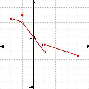
Example1.5
Consider the function \(f(x)\) graphed below. Figure1.6Graph of \(y =f(x)\) For the function \(f\) pictured in Figure1.6, we make the following observations:
When finding a limit from a graph, it suffices to ask if the function approaches a single value from each side of the fixed input. The function value at the fixed input is irrelevant. Thus, the limit to \(-1\) is \(3\) even though \(f(-1)=4\) (where the filled in dot is), and the limit to \(3\) is \(-1\) even though \(f(3)=DNE\text{.}\) This reasoning explains the values of the four limits stated above.
We further observe that \(f\) does not have a limit as \(x\) approaches \(1\) because there is a jump in the graph at \(x = 1\text{.}\) If we approach \(x = 1\) from the left, the function values tend to get close to \(-1\text{,}\) but if we approach \(x = 1\) from the right, the function values get close to 0. There is no single number that all of these function values approach. This is why the limit of \(f\) does not exist at \(x = 1\text{.}\)
Limits have some useful properties with respect to algebraic operations. These are stated below as we will take advantage of them in future sections.
Properties of Limits
Assuming \(\lim\limits_{x \rightarrow c} f(x) = L \) and \(\lim\limits_{x \rightarrow c} g(x) = M\) for real numbers \(L \) and \(M \) we have that the following are true.
If \(b\) is a constant, then \(\lim\limits_{x \rightarrow c} (bf(x))=b\left(\lim\limits_{x \rightarrow c} f(x) \right)=b\cdot L\)
\(\lim\limits_{x \rightarrow c} \left( f(x)\pm g(x)\right)=\lim\limits_{x \rightarrow c} f(x)\pm\lim\limits_{x \rightarrow c}g(x) = L \pm M \)
\(\lim\limits_{x \rightarrow c} \left( f(x) \cdot g(x)\right)=\lim\limits_{x \rightarrow c} f(x)\cdot\lim\limits_{x \rightarrow c}g(x) = L \cdot M \)
\(\lim\limits_{x \rightarrow c} \left[ \left(f(x)\right)^n \right] = \left[ \lim\limits_{x \rightarrow c} f(x) \right]^n = L^n \) for \(n>0\) provided \(L^n \) is a real number
For any constant \(k\text{,}\) \(\lim\limits_{x \rightarrow c} k=k\)
\(\lim\limits_{x \rightarrow c} x=c\)
SubsectionSummary
For a function \(f\) defined on an interval around a number \(c\text{,}\)
means that the value of \(f(x)\) gets as close as we want to a number \(L\) whenever \(x\) is sufficiently close to \(c\text{,}\) assuming the value \(L\) exists.
We define a limit from the left and a limit from the right in the same way as above, while adding the stipulation that \(x\lt c\) for the left limit and \(x\gt c\) for the right limit. That is, as we move \(x\) sufficiently close to \(c\) from the left on a number line (\(x\lt c\)), \(f(x)\) gets as close to the limit value as we want. Similarly for the limit from the right.
A function \(f\) has limit \(L\) as \(x \to a\) if and only if \(f\) has a left-hand limit at \(x = a\text{,}\) \(f\) has a right-hand limit at \(x = a\text{,}\) and the left- and right-hand limits are equal. Visually, this means that there can be a hole in the graph at \(x = a\text{,}\) but the function must approach the same single value from either side of \(x = a\text{.}\)